Page 224 - Modern Control Systems

198 Chapter 3 State Variable Models

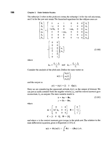
The subscript 2 refers to the pitch axis terms, the subscript 1 is for the roll axis terms,
and 3 is for the yaw axis terms. The linearized equations for the roll/yaw axes are
~*r 0 n I 0 0 0~ "V

03 —n 0 0 1 0 0 03
2
wj 3« A, 0 0 -«A t 0 0 (D X
=
w 3 0 0 -«A 3 0 0 0 w 3
k 0 0 0 0 0 n hi
0 0 0 0 —n 0_
> 3 _ Jh.

0 o"
0 0
l 0
+ A l i (3.100)
0
h _« 3_
1 0
0 1_
where
h - 1 h ~h
A, := an A A

Consider the analysis of the pitch axis. Define the state-vector as
(0 2(t)\
x(t) := a> 2(t) ,
VMO/
and the output as
y(t) = d 2(T) = [1 0 0]x(f).
Here we are considering the spacecraft attitude, ^2(0^ a s t n e output of interest. We
can just as easily consider both the angular velocity, w 2 > and the control moment gyro
momentum, h 2, as outputs. The state variable model is
x = Ax + Bit, (3.101)
y = Cx + Du,
where
0 1 o" " 0
A = 2 A 2 0 0 , B = 1
h
0 0 0_ _ 1 _
C = [1 0 0], D = [0],
and where it is the control moment gyro torque in the pitch axis. The solution to the
state differential equation, given in Equation (3.101), is

\(t) = 3>(f)x(0) + / *(* - T)BU(T) dr,