Page 225 - Modern Control Systems

Section 3.8 Design Examples 199

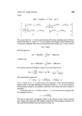
where

-1
l
¢(0 = exp(Af) = C~ {(sl - A) }

2 2
2 V3« A 2

0 0 1

We can see that if A 2 > 0, then some elements of the state transition matrix will have
al
terms of the form e , where a > 0. As we shall see (in Chapter 6) this indicates that
our system is unstable. Also, if we are interested in the output, y(t) = 02(0» w e n a v e
y{t) = Cx(0.
With x(r) given by

x(0 = *(0x(0) + / <D(f - T)Bu(T)dT,
Jo
it follows that

y(t) = C<D(0x(0) + [ C<D(/ - T)Bu{r)dr.
Jo
The transfer function relating the output Y(s) to the input U(s) is

n*) „,. . i
B
G s C sl A W n
( ) = 777T = ( v ~ ) = " 2 2
U(s) ' / 2(s - 3« A 2)
The characteristic equation is
2 2 2 2
s - 3« A 2 = (s + V3n A 2)(s - V3n A 2) = 0.
If A 2 > 0 (that is, if / 3 > I\), then we have two real poles—one in the left half-plane
and the other in the right half-plane. For spacecraft with I 3 > I h we can say that an
earth-pointing attitude is an unstable orientation. This means that active control is
necessary.
Conversely, when A 2 < 0 (that is, when I x > / 3 ), the characteristic equation has
two imaginary roots at

2
s = ±;V3n |A 2|.
This type of spacecraft is marginally stable. In the absence of any control moment
gyro torques, the spacecraft will oscillate around the earth-pointing orientation for
any small initial deviation from the desired attitude. •