Page 230 - Modern Control Systems

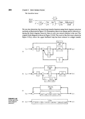
204 Chapter 3 State Variable Models

We therefore have

-.J is
*(*)
Us) , (b 2k 2kr 2 2kb 2kK„,k 1k 2r
+ — + —— )s + Jm JmR
m J
We can also determine the closed-loop transfer function using block diagram reduction
methods, as illustrated in Figure 3.32. Remember, there is no unique path to follow in re-
ducing the block diagram; however, there is only one correct solution in the end. The
original block diagram is shown in Figure 3.31(b). The result of the first step is shown in
Figure 3.32(a), where the upper feedback loop has been reduced to a single transfer

Us *> Xf(s)
(a)

2kK mk 2k x
mRs
' — 1 mrs
(b) 7 » ~^ t 2 •+-XA.S)
J s ms + 2k
• * > i , -
b Ihnrs
+ 2
J J(ms + 2k)

2kK mk 2ki
mRs
(c)
1
*
2
T/s) + Q Jtm* + mbs 2 + 2k(J + mr )s + 2bk * — • X . ( s )
FIGURE 3.32
Printer belt drive -(r/J)s
block diagram (d) T/s) 2 2 X,(s)
reduction. s* + {b/J)s + Qk/m + 2kr /J)s + 2bk/(Jm) + 2rkK ink 2k i/(mJR)