Page 232 - Modern Control Systems

206 Chapter 3 State Variable Models

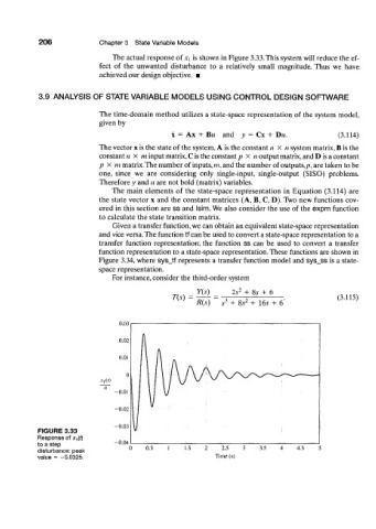
The actual response of X\ is shown in Figure 3.33. This system will reduce the ef-
fect of the unwanted disturbance to a relatively small magnitude. Thus we have
achieved our design objective. •

3.9 ANALYSIS OF STATE VARIABLE MODELS USING CONTROL DESIGN SOFTWARE

The time-domain method utilizes a state-space representation of the system model,
given by
x = Ax + BM and v = Cx + T>u. (3.114)
The vector x is the state of the system, A is the constant n X n system matrix, B is the
constants X m input matrix, C is the constant p X n output matrix, and D is a constant
p X m matrix.The number of inputs, m, and the number of outputs,p, are taken to be
one, since we are considering only single-input, single-output (SISO) problems.
Therefore y and u are not bold (matrix) variables.
The main elements of the state-space representation in Equation (3.114) are
the state vector x and the constant matrices (A, B, C, D). Two new functions cov-
ered in this section are ss and Isim. We also consider the use of the expm function
to calculate the state transition matrix.
Given a transfer function, we can obtain an equivalent state-space representation
and vice versa. The function tf can be used to convert a state-space representation to a
transfer function representation; the function ss can be used to convert a transfer
function representation to a state-space representation. These functions are shown in
Figure 3.34, where sys_tf represents a transfer function model and sys_ss is a state-
space representation.
For instance, consider the third-order system
Y(s) 2s 2 + 8A- + 6
T(s) 2 (3.115)
R(s) A- + 8.v + 16.v + 6'
3

FIGURE 3.33
Response of x^f)
to a step
disturbance: peak
value = -0.0325.