Page 235 - Modern Control Systems

Section 3.10 Sequential Design Example: Disk Drive Read System 209

»A=[0 -2; 1 -3]; dt=0.2; Phi=expm(A*dt)

FIGURE 3.37 Phi =
Computing the
state transition 0 9671 0 2968 4 - State transition matrix
matrix for a given 0.1484 0.5219 for a At of 0.2 second
time, At = dt.

The initial conditions are -Vi(0) = ^(0) = 1 and the input u(t) = 0. At t = 0.2, the
state transition matrix is as given in Figure 3.37. The state at t = 0.2 is predicted by
the state transition methods to be

0.9671 -0.2968 0.6703
x {
x-> /=0.2 0.1484 0.5219 /=0 0.6703
The time response of the system of Equation (3.115) can also be obtained by
using the Isim function. The Isim function can accept as input nonzero initial condi-
tions as well as an input function, as shown in Figure 3.38. Using the Isim function, we
can calculate the response for the RLC network as shown in Figure 3.39.
The state at t = 0.2 is predicted with the Isim function to be ^(0.2) = x 2(0.2) =
0.6703. If we can compare the results obtained by the Isim function and by multiplying
the initial condition state vector by the state transition matrix, we find identical results.

3.10 SEQUENTIAL DESIGN EXAMPLE: DISK DRIVE READ SYSTEM

Advanced disks have as many as 5000 tracks per cm. These tracks are typically
1 [xm wide. Thus, there are stringent requirements on the accuracy of the reader
head position and of the movement from one track to another. In this chapter, we

u(1) v(0
A System
Arbitrary
x = Ax + B/( Output
input
v = Cx + DM
• > /
(a)

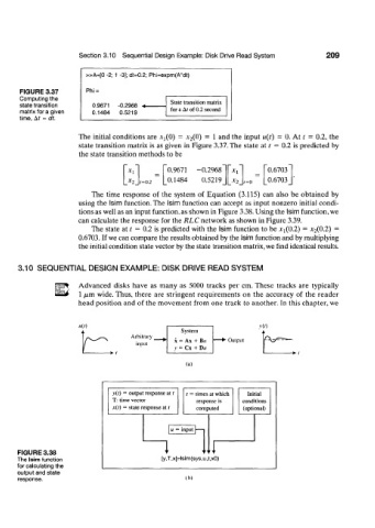
y(t) = output response at t t = times at which Initial
T: time vector response is conditions
A(r) = state response at t computed (optional)

u = input

FIGURE 3.38
The Isim function [y,T,x]=lsim(sys,u,t,xO)
for calculating the
output and state
response. (b)