Page 239 - Modern Control Systems

Section 3.11 Summary 213

% Model Parameters
k=10; Units
M 1=0.02; M2=0.0005; k: kg/m
b: kg/m/s
D1—41 Ue-UJ, D^—4.1 e-Uo, *
t=[0:0.001:1.5]; m:kg
% state apace Moael
A=[0 0 1 0;0 0 0 1;-k/M1 k/M1 -b1/M1 0; k/M2 -k/M2 0 -b2/M2];
B=[0;0;1/M1;0]; C=[0 0 0 1]; D=[0j; sys=ss(A,B,C,D);
% Simulated Step Response
y=step(sys,t); plot(t,y); grid
xlabel(Time (s)'), ylabel('y dot (m/s)')

3
I
2.5
AAA
2
1
r i.5 Mass 2
o
position rate
1
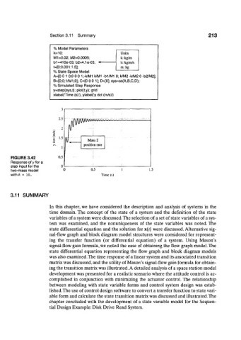
FIGURE 3.42 0.5 -- | -
Response of y for a
step input for the 0 i
two-mass model 0.5 1 1.5
with/c = 10. Time (s)

3.11 SUMMARY

In this chapter, we have considered the description and analysis of systems in the
time domain. The concept of the state of a system and the definition of the state
variables of a system were discussed. The selection of a set of state variables of a sys-
tem was examined, and the nonuniqueness of the state variables was noted. The
state differential equation and the solution for x(t) were discussed. Alternative sig-
nal-flow graph and block diagram model structures were considered for represent-
ing the transfer function (or differential equation) of a system. Using Mason's
signal-flow gain formula, we noted the ease of obtaining the flow graph model. The
state differential equation representing the flow graph and block diagram models
was also examined. The time response of a linear system and its associated transition
matrix was discussed, and the utility of Mason's signal-flow gain formula for obtain-
ing the transition matrix was illustrated. A detailed analysis of a space station model
development was presented for a realistic scenario where the attitude control is ac-
complished in conjunction with minimizing the actuator control. The relationship
between modeling with state variable forms and control system design was estab-
lished. The use of control design software to convert a transfer function to state vari-
able form and calculate the state transition matrix was discussed and illustrated. The
chapter concluded with the development of a state variable model for the Sequen-
tial Design Example: Disk Drive Read System.