Page 236 - Modern Control Systems

210 Chapter 3 State Variable Models

0 0.1 0.2 0.3 0.4 0.5 0.6 0.7 0.8 0.9 1.0 0 0.1 0.2 0.3 0.4 0.5 0.6 0.7 0.8 0.9 1.0
Time (s) Time (s)

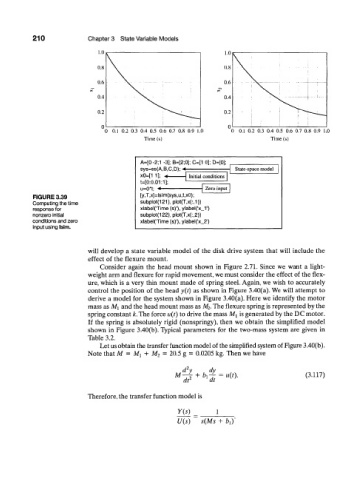
A=[0-2;1 -3]; B=[2;0]; C=[1 0]; D=[0];
sys=ss(A,B,C,D); * State-space model
x0=[1 1]; A Initial conditions
t=[0:0.01:1];
u=0*t; * Zero input
FIGURE 3.39 [y,T,x]=lsim(sys,u,t,xO);
Computing the time subplot(121), plot(T,x(:,1))
response for xtabel(Time (s)'), ylabel('x_1')
nonzero initial subplot(122),p!ot(T,x(:,2))
conditions and zero xlabel('Time (s)'), ylabel('x_2')
input using Isim.

will develop a state variable model of the disk drive system that will include the
effect of the flexure mount.
Consider again the head mount shown in Figure 2.71. Since we want a light-
weight arm and flexure for rapid movement, we must consider the effect of the flex-
ure, which is a very thin mount made of spring steel. Again, we wish to accurately
control the position of the head y(t) as shown in Figure 3.40(a). We will attempt to
derive a model for the system shown in Figure 3.40(a). Here we identify the motor
mass as Mi and the head mount mass as M 2 . The flexure spring is represented by the
spring constant A:. The force u(t) to drive the mass M x is generated by the DC motor.
If the spring is absolutely rigid (nonspringy), then we obtain the simplified model
shown in Figure 3.40(b). Typical parameters for the two-mass system are given in
Table 3.2.
Let us obtain the transfer function model of the simplified system of Figure 3.40(b).
Note that M = M l + M 2 = 20.5 g = 0.0205 kg. Then we have

2
d y dy
M-j + bi— = u(t). (3.117)
at dt
Therefore, the transfer function model is

Y(s) 1
U(s) s(Ms + bi)'