Page 231 - Modern Control Systems

Section 3.8 Design Examples 205

function. The second step illustrated in Figure 3.32(b) then reduces the two lower feed-
back loops to a single transfer function. In the third step shown in Figure 3.32(c), the lower
feedback loop is closed and then the remaining transfer functions in series in the lower
loop are combined. The final step closed-loop transfer function is shown in Figure 3.32(d).
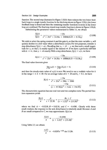
Substituting the parameter values summarized in Table 3.1, we obtain
Ai(j) -15.9
* v ' = i ± ! /3 1 QO\
2
3
T d(s) 5 + 25s + 14.5^ + 1000A:(0.25 + 0.15^)' '
We wish to select the spring constant k and the gain k 2 so that the state variable X\ will
quickly decline to a low value when a disturbance occurs. For test purposes, consider a
step disturbance T d(s) = a/s. Recalling that x\ = rd — y, we thus seek a small magni-
tude for X] so that y is nearly equal to the desired rO. If we have a perfectly stiff belt
with k —* 00, then y = rO exactly. With a step disturbance, 7^(5) = a/s, we have

-15a
*(*) = 3 ^ 2 2 • « , . . . , ^ . • - ^ . , - (3.109)
3
5 + 25s + 14.5*5 + 1000A:(0.25 + 0.15^)
The final value theorem gives
limjc^f) = limsX^s) = 0, (3.110)
t—»00 s—*0
and thus the steady-state value of xi(t) is zero. We need to use a realistic value for k
in the range 1 < A: < 40. For an average value of k = 20 and k 2 = 0.1, we have

Ms) = - f^
2
5 3 + 25s + 2905 + 5300
~15a
(5 + 22.56)(5 2 + 2.445 + 234.93) (3.111)
The characteristic equation has one real root and two complex roots. The partial frac-
tion expansion yields

m = _ ^ _ + i£±C - 2 , (3.112)
2
a s + 22.56 (5 + 1.22) + (15.28) 2 V
where we find A = -0.0218,5 = 0.0218, and C = -0.4381. Clearly with these
small residues, the response to the unit disturbance is relatively small. Because A and
B are small compared to C, we may approximate X\(s) as

X x{s) -0.4381
2
2
a (5 + 1.22) + (15.28) '
Using Table 2.3, we obtain

x\(t) -L22
= -0.0287e ' sin 15.28/. (3.113)