Page 233 - Modern Control Systems

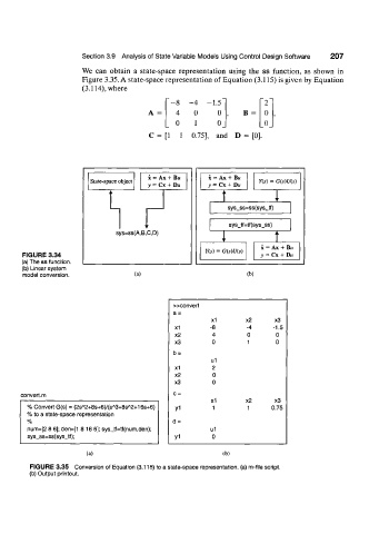
Section 3.9 Analysis of State Variable Models Using Control Design Software 2 0 7

We can obtain a state-space representation using the ss function, as shown in
Figure 3.35. A state-space representation of Equation (3.115) is given by Equation
(3.114), where
8 -4 -1.5 2
4 0 0 B = 0
0 1 0_ _()
C = [l 1 0.75], and D = [0]

x = Ax + B« x = Ax + BH
State-space object Y(s) = G(s)U(s)
y = Cx + DK y = Cx + DH
i L i i
T
sys_ss=ss(sys_tf)

sys_tf=tf{sys_ss)
S! fS=SS (A B, C,D) i L
ir
x = Ax + BH
Y(s) = G{s)U(s)
FIGURE 3.34 y = Cx + DH
(a) The ss function.
(b) Linear system
model conversion. (a) (b)

»convert
a =
x1 x2 x3
X1 -8 -4 -1.5
x2 4 0 0
x3 0 1 0
b =
u1
x1 2
x2 0
x3 0
convert, m c =
x1 x2 x3
A
A
A
% Convert G(s) = (2s 2+8s+6)/(s 3+8s 2+16s+6) yi 1 1 0.75
% to a state-space representation
% d =
num=[2 8 6]; den=[1 8 16 6]; sys_tf=tf(num,den); u1
sys_ss=ss(sys_tf); y1 0
(a) (b)

FIGURE 3.35 Conversion of Equation (3.115) to a state-space representation, (a) m-file script.
(b) Output printout.