Page 238 - Modern Control Systems

212 Chapter 3 State Variable Models

d y dy
J
Mass M>: M 2- j + b 2-j- + k(y - q) = 0.
dt dt
To develop the state variable model, we choose the state variables as x\ = q and
= y. Then we have
,v 2
dq dy
x-i = — a n d A'4 = —-.
dt dt
Then, in matrix form,

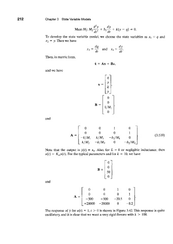
x = Ax + Bw,
and we have

<1
y
q
y
o
B= °
1/Afi
0
and

0 0 1 0
0 0 0 1
A = (3.119)
-klM x 0
0
k/M 2 -k/M 2 ~b 2/M 2
Note that the output is y(t) = x 4. Also, for L = 0 or negligible inductance, then
u(t) = K mv(t). For the typical parameters and for k = 10, we have

0
0
B =
50
0_
and
0 0 1 0
0 0 0 1
A =
-500 +500 -20.5 0
+20000 -20 000 0 -8.2
The response of y for u(t) = 1, t > 0 is shown in Figure 3.42. This response is quite
oscillatory, and it is clear that we want a very rigid flexure with k > 100.