Page 234 - Modern Control Systems

208 Chapter 3 State Variable Models

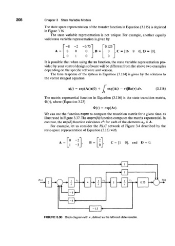
The state-space representation of the transfer function in Equation (3.115) is depicted
in Figure 3.36.
The state variable representation is not unique. For example, another equally
valid state variable representation is given by

-2 -0.75" ' 0.125"
A = 0 0 ,B = 0 , C = [16 8 6], D = [0).
0 1 0 0
It is possible that when using the ss function, the state variable representation pro-
vided by your control design software will be different from the above two examples
depending on the specific software and version.
The time response of the system in Equation (3.114) is given by the solution to
the vector integral equation

x(0 = exp(Af)x(0) + / exp[A(r - T)]BW(T) dr. (3.116)
Jo
The matrix exponential function in Equation (3.116) is the state transition matrix,
$(f), where (Equation 3.23)

¢(0 = exp(Ar)-
We can use the function expm to compute the transition matrix for a given time, as
illustrated in Figure 3.37. The expm(A) function computes the matrix exponential. In
a,
contrast, the exp(A) function calculates e > for each of the elements a i} E A.
For example, let us consider the RLC network of Figure 3.4 described by the
state-space representation of Equation (3.18) with

0 -2 2
A = B = C = [1 0], and D = 0.
i -3 0

K(v)

FIGURE 3.36 Block diagram with x : defined as the leftmost state variable.