Page 288 - Phase-Locked Loops Design, Simulation, and Applications

MIXED-SIGNAL PLL APPLICATIONS PART 2: FRACTIONAL-N FREQUENCY
SYNTHESIZERS Ronald E. Best 171
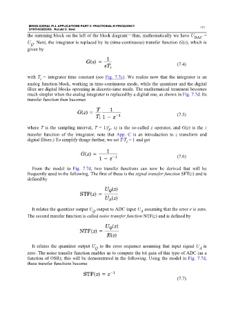
the summing block on the left of the block diagram—thus, mathematically we have U DAC =
U . Next, the integrator is replaced by its (time-continuous) transfer function G(s), which is
Q
given by

(7.4)

with T = integrator time constant (see Fig. 7.7c). We realize now that the integrator is an
i
analog function block, working in time-continuous mode, while the quantizer and the digital
filter are digital blocks operating in discrete-time mode. The mathematical treatment becomes
much simpler when the analog integrator is replaced by a digital one, as shown in Fig. 7.7d. Its
transfer function then becomes

(7.5)

where T is the sampling interval, T = 1/f . (z is the so-called z operator, and G(z) is the z
F
transfer function of the integrator; note that App. C is an introduction to z transform and
digital filters.) To simplify things further, we set T/T = 1 and get
i

(7.6)

From the model in Fig. 7.7d, two transfer functions can now be derived that will be
frequently used in the following. The first of these is the signal transfer function SFT(z) and is
defined by

It relates the quantizer output U output to ADC input U assuming that the error e is zero.
Q
A
The second transfer function is called noise transfer function NTF(z) and is defined by

It relates the quantizer output U to the error sequence assuming that input signal U is
A
Q
zero. The noise transfer function enables us to compute the bit gain of this type of ADC (as a
function of OSR); this will be demonstrated in the following. Using the model in Fig. 7.7d,
these transfer functions become

(7.7)