Page 81 - Photodetection and Measurement - Maximizing Performance in Optical Systems

Fundamental Noise Basics and Calculations

74 Chapter Three

1
0.9
Clock frequency/
0.8
sequence length
0.7
Amplitude 0.5
0.6

0.4
0.3 Clock frequency
0.2
0.1
0
0 20 40 60 80 100
Frequency
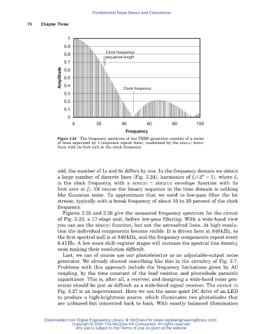
Figure 3.24 The frequency spectrum of the PRBS generator consists of a series
of lines separated by 1/(sequence repeat time), modulated by the sinc(x) wave-
form with its first null at the clock frequency.

odd, the number of 1s and 0s differs by one. In the frequency domain we obtain
N
a large number of discrete lines (Fig. 3.24), harmonics of f C /(2 - 1), where f C
is the clock frequency, with a sinc(x) = sin(x)/x envelope function with its
first zero at f C . Of course the binary sequence in the time domain is nothing
like Gaussian noise. To approximate that we need to low-pass filter the bit
stream, typically with a break frequency of about 10 to 20 percent of the clock
frequency.
Figures 3.25 and 3.26 give the measured frequency spectrum for the circuit
of Fig. 3.23, a 17-stage unit, before low-pass filtering. With a wide-band view
you can see the sinc(x) function, but not the unresolved lines. At high resolu-
tion the individual components become visible. It is driven here at 840kHz, so
the first spectral null is at 840kHz, and the frequency components repeat every
6.41Hz. A few more shift-register stages will increase the spectral line density,
soon making their resolution difficult.
Last, we can of course use our photodetector as an adjustable-output noise
generator. We already showed something like this in the circuitry of Fig. 3.7.
Problems with this approach include the frequency limitations given by AC
coupling, by the time constant of the load resistor, and photodiode parasitic
capacitance. This is, after all, a receiver, and designing a wide-band noise gen-
erator should be just as difficult as a wide-band signal receiver. The circuit in
Fig. 3.27 is an improvement. Here we use the same quiet DC drive of an LED
to produce a high-brightness source, which illuminates two photodiodes that
are unbiased but connected back to back. With exactly balanced illumination

Downloaded from Digital Engineering Library @ McGraw-Hill (www.digitalengineeringlibrary.com)
Copyright © 2004 The McGraw-Hill Companies. All rights reserved.
Any use is subject to the Terms of Use as given at the website.