Page 215 - Pipeline Risk Management Manual Ideas, Techniques, and Resources

8/192 Data Management and Analyses
over time is shown. Trends can therefore be spotted that is, “In HLC charts
which direction and by what magnitude are things changing
over time?” Used in conjunction with the histogram, where the A charting technique borrowed from stock market analysis, the
evaluator can see the shape of the data, information and pat- high-low-close (HLC) chart (Figure 8.5) is often used to show
terns ofbehavior become more available. daily stock share price performance. For purposes of risk score
analysis, the average will be substituted for the “close” value.
Correlation charts This chart simultaneously displays a measure of central ten-
dency and the variation. Because both central tendency and
Of special interest to the risk manager are the relationships variation are best used together in data analysis, this chart pro-
between risk variables. With risk variables including attributes, vides a way to compare data sets at a glance.
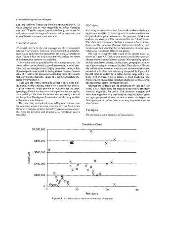
preventions, and costs, the interactions are many. A correlation One way to group the data would be by system name, as
chart (Figure 8.4) is one way to qualitatively analyze the extent shown in Figure 8.5. Each system name contains the scores of
of the interaction between two variables. all pipeline sections within that system. Other grouping options
Correlation can be quantified but for a rough analysis, the include population density, product type, geographic area, or
two variables can be plotted as coordinates on an x,y set of axes. any other meaningful slicing ofthe data. These charts will visu-
If the data are strongly related (highly correlated), a single line ally call attention to central tendencies or variations that are not
ofplotted points is expected. In the highest correlation, for each consistent with other data sets being compared. In Figure 8.5,
value ofx, there is one unique corresponding value ofy. In such the AB Pipeline system has a rather narrow range and a rela-
high correlation situations, values of y can be accurately pre- tively high average. This is usually a good condition. The
dicted from values ofx. Frijole Pipeline has a large variation among its section scores,
If the data are weakly correlated, scatter is seen in the plot- and the average seems to be relatively low.
ted points. In this situation, there is not a unique y for every x. Because the average can be influenced by just one low
A given value of x might provide an indication for the corre- score, a HLC chart using the median as the central tendency
sponding y if there is some correlation present, but the predic- measure might also be useful. The observed averages and
tive capability of the chart diminishes with increasing scatter of variations might be easily explained by consideration of prod-
the data points. The degree of correlation can also be quantified uct type, geographical area, or other causes. An important
with numerical techniques. finding may occur when there is no easy explanation for an
There are many examples of expected high correlation: coat- observation.
ing condition versus corrosion potential, activity level versus
third-party damage, product hazard versus leak consequences, Examples
etc. Both the presence and absence of a correlation can be
revealing. We now look at some examples of data analysis.

Correlation Chart
$1,000,000
X

s X
$800,000 X

X
$600,000
0”
-
a
c x X .I x
2 $400,000
xx XX
x ., xex
$200,000
X
xyx X
0- I
0 50 100 150
Risk Score
Figure 6.4 Correlation chart: risk score versus costs of operation.