Page 297 - Pipeline Risk Management Manual Ideas, Techniques, and Resources

13/274 Stations and Surface Facilities
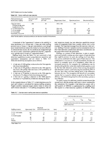
Table 13.6 Station staffing for leak detection
Field operations and Hoursper week Inspection hours
maintenance staffing on site per week Happenstance hours Opportunity hours Max interval hours
7 days per week x 168 84 50% x 168 168 2
24 hours per day, with
rounds (every 2 hr)
5 x 8, with rounds (2 hr) 40 20 50% x 40 40 60
7 x 24, no rounds I68 0 50% x I68 84 10 est.
5 x 8, no rounds 40 0 50%x40 20 60
Once/week, 2 hr on site 2 2 50% x 2 3 I66
Nofe: Partial credit for remote surveillance can also be included in this scheme.

A drawback of the “opportunity” scheme is the inability to mal inspection rounds, has leak detection capabilities several
show preference of a 1 hr per day x 5 days per week staffing orders of magnitude better than a weekly station visit, in this
protocol over a 5 hours x 1 day per week protocol, even though example. The important message from this exercise is that vari-
most would intuitively believe the former to be more effective. ous ‘staffing of stations’ scenarios can be evaluated in terms of
To obtain the best results, the two methods are merged through their leak detection contributions and those contributions can
the use of a ratio: (maximum unobserved interval) / (opportu- be a part of the overall risk assessment.
nity), and this ratio is in units of “opportunity-hours.” Staffing, as a means of leak detection, is seen to supple-
Staffing levels from the Table 13.6 are converted to leak ment and partially overlap any other means of leak detection
detection capabilities (scores) using detection sensitivity and that might be present. As such, the staffing level leak detec-
opportunity assumptions and are shown in Table 13.7. tion can be combined with other types of leak detection. The
Detection sensitivity assumptions are as follows: combination is not seen as a straight summation, because the
benefit is normally more of a redundancy rather than an
1. A leak rate of 1000 galiday is detected on the first opportu- increased sensitivity. For example, the combination can be
nity-hour (immediately). done by taking the best value (the smallest leak quantity, as set
2. A leak rate of 100 gal/day is detected on the 10th opportu- by the best leak detection system) from among the parallel
nity-hour (100 gaVday leak rates have a 10% probability of leak detection systems, and improving that number by 50% of
detection during any hour). the next best value and then adding back in the difference
3. A leak rate of 10 gal/day is detected on the 50th opportu- between the two. This recognizes the benefit of a secondary
nity-hour (a 2% chance of detection during any hour). system that is as good or almost as good as the first line of
4. A leak rate of 1 gaUday is detected on the 100th opportu- defense, with diminishing benefit as the secondary system is
nity-hour (a 1% probability of detection during any hour). less effective.
No credit is given for additional parallel systems beyond the
In the example shown in Table 13.7, a leak detection score for second level, and the primary spill score is never worsened by
each spill volume is calculated for various staffing scenarios. this calculation. For example, a leak detection system with a
Higher numbers represent longer relative times to detect the spill quantity of 3000 bbl is supplemented by a staffing level
spill volume indicated. A 7-24 staffing arrangement, with for- that equates to a leak detection capability of 2000 bbl. When
Table 13.7 Example station staffing leak detection capabilities

Leak rate detection scores

Assumed detection sensitivity (opportunity hours
before detection)
Maximum
Staffingscenario OpportunirJP fir) unobserved timC (hr) Ratio 100 50 IO I
7 x 24, with rounds 168 2 0.01 1 0.5 0.1 0.01
7x24 84 10 0.11 11 6 1.1 0.11
5 x 8 with rounds
40 60 1.5 150 75 15 1.5
5x8 20 60 3.0 300 150 30 3.0
Weekly 3 166 55.3 5530 2765 553 55.3
#SeeTable 13.6.