Page 342 - Pipeline Risk Management Manual Ideas, Techniques, and Resources

Case studies 14/319
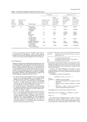
Table 2 Calculated Post-Mitigation Probabilities of Selected Impacts

Overall Risk Segmenr-Specific RI rk
Annual Prohahilit? Annual
prohubr1ih;f ofone or more prf~habikiy
Averuge Predicted Leak Pmhubilih; ofone one or more evenfs over the (done or more
Leak Countfor or more events events during lfeofthe evenh during
Rate per 700 Miles over the life of the life of the project !he lifi ofthe
Mile-Year and 50 Years Porentinl Impact theproject (%) project (%J (W projecf l%)
0.00007 2.6 Dnnking water 0.5 0.0 I0 0.00035 0 00001
contamination
Drinking water, 0.3 0.005 0.00017 0.000004
no MTBE
Fatality 0.5 0.01 1 0.00036 0.00001
Injury 2.3 0.047 0.00 160 0.00003
Recreational 8.3 0.17 0.006 0.000 12
water
contamination
Prime agricultural 3.5 0.070 0.002 0.00005
contamination
Wetlands contamination 4.9 0.10 0.005 0.00009
Lake Travis drinking 0.02 0.0004 0.000013 0 oooooo26
water supply
Edwards Aquifer 0.02 0.0004 0.000013 0.00000026
water contamination

operation and maintenance activities. “Receptors” refer to the sites & ~ ~~ ~ ~ ~
or organisms that are threatened by a spill of refined products. Index Sum Pmbabilip ofLeak (e.\rimated by frequen<:v in w7it.s of
Receptors in this report include people, drinking water supplies, and leaks per mileyear)
wetlands. Each impact potentially damages one or more receptors.
0 1 .0 (100 percent chance ofa leak)
189 0.00199 (historical EPC leak rate on this pipeline)
Leak Frequencies 400 0 (virtually no chance of a leak)
Pipeline leak frequencies are estimated from several data sources. Four Note that this exercise does not create a curve that passes exactly
(4)“frequencyofleak”casesare examinedinthisreport. Eachcase rep- through each of these points. In fact, the curve that best fits all points
resents a different estimated incident rate and is used independently to actually passes through a point that represents a mitigation-effect
perform an impacts assessment. Three cases use only historical data level of90 to 95 percent.
with no consideration given to possible benefits ofmitigation. These are For Cases 3 and 4, leak probabilities are calculated in addition
included for reference and represent impact frequencies that might be to leak frequencies. These are obtained by calculating the Poisson
seen on an unmitigated LPP pipeline and on a typical US hazardous probability estimate of“one or more” leaks over the life ofthe project,
liquid pipeline. The fourth case considers the effects of mitigation. The as shown below.
four leak frequencies are generally described as follows: The probability ofno spills is calculated from.
Case I (all US. hazardous liquidpipeline leak rate): The average leak P(x)sPILL=[(~’~)x:x!]*~~~(-~‘~~
incident rate for reportable accidents on US hazardous liquids where
pipelines, from 1968&1999(DOT, 1999 andinEAChapter5). P(X)SPILL = probability ofexactly X spills
Case 2 former EPCpipeline, reportable leak rate): The reportable f = the average spill frequency for a segment of interest.
incident (i.e., accidents in which spill volumes were 50 barrels or spills /year
more) rate for 450 miles ofthis pipeline under EPC operation in 29 t = the time period for which the probability is sought.
years. (Incident rate) = (10 leaks) / (450 miles x 29 years). years
Case 3 former EPCpipeline, overall leak rate): The overall incident X = the number of spills for which the probability is
rate, regardless of spill size, for 450 miles of pipeline (not including sought. in the pipeline segment of interest
pump stations) under EPC operations in 29 years. (Incident rate) =
(26leaks)/(450milesx29years). The probability for one or more spills is evaluated as follows:
Case 4 (uses an estimate of mitigation efeects plus historical data):
Cases 1-3 use leak frequencies that do not consider index sums and P(probabi1ity of one or more)SPILL = I - Probablhty of no spills =
hence do not consider effects of mitigation. In case 4, distinctions 1 -P(X)SPILL
are made regarding the impacts of mitigation for the various tier where X = 0.
categories or for a specific geographic area. The corresponding
index sum is used to estimate a leak frequency. The leak frequency The results of these calculations are shown in Table 2 (Executive
is therefore estimated by correlating the index sum scale to an Summary) and in Tables 5 through 8 [Tables 7 and R not included in
absolute leak frequency. The correlating equation used represents this hook]. The leak frequency estimates have a high degree ofuncer-
the curve that best fits the following points: tainty, primarily due to the limited amount of data available No data