Page 115 - Power Electronic Control in Electrical Systems

//SYS21/F:/PEC/REVISES_10-11-01/075065126-CH003.3D ± 103 ± [82±105/24] 17.11.2001 9:53AM

Power electronic control in electrical systems 103

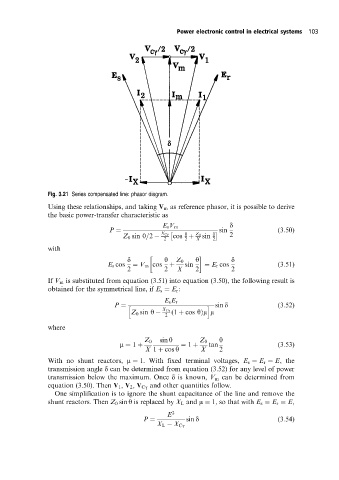
Fig. 3.21 Series compensated line: phasor diagram.

Using these relationships, and taking V m as reference phasor, it is possible to derive
the basic power-transfer characteristic as
d
E s V m
P ˆ sin (3:50)
X Cg y Z 0 y 2
Z 0 sin y=2 cos ‡ sin
2 2 X 2
with
d y Z 0 y d
E s cos ˆ V m cos ‡ sin ˆ E r cos (3:51)
2 2 X 2 2
If V m is substituted from equation (3.51) into equation (3.50), the following result is
obtained for the symmetrical line, if E s ˆ E r :

E s E r
i sin d (3:52)
P ˆ h
X Cg
Z 0 sin y (1 ‡ cos y†m m
2
where
Z 0 sin y Z 0 y
m ˆ 1 ‡ ˆ 1 ‡ tan (3:53)
X 1 ‡ cos y X 2
With no shunt reactors, m ˆ 1. With fixed terminal voltages, E s ˆ E r ˆ E, the
transmission angle d can be determined from equation (3.52) for any level of power
transmission below the maximum. Once d is known, V m can be determined from
equation (3.50). Then V 1 , V 2 , V Cg and other quantities follow.
One simplification is to ignore the shunt capacitance of the line and remove the
shunt reactors. Then Z 0 sin y is replaced by X L and m ˆ 1, so that with E s ˆ E r ˆ E,
E 2
P ˆ sin d (3:54)
X L X Cg