Page 129 - Power Electronic Control in Electrical Systems

//SYS21/F:/PEC/REVISES_10-11-01/075065126-CH004.3D ± 117 ± [106±152/47] 17.11.2001 9:54AM

Power electronic control in electrical systems 117
1
where V ˆ V l V m and Y k ˆ .
Z k
The injected nodal current at node i may be expressed as a function of the currents
entering and leaving the node through the q branches connected to the node
q
X
I i ˆ I k (4:16)
kˆ1
where I i is the nodal current at node i and branch k is connected to node i. Also, I k is
the current in branch k.
Combining equations (4.15) and (4.16) leads to the key equation used in nodal
analysis
q
X
I i ˆ Y k (V l V m ) (4:17)
kˆ1
which can also be expressed in matrix form for the case of n nodes
2 3 2 32 3
I 1 Y 11 Y 12 Y 13 Y 1n V 1
I 2 Y 21 Y 22 Y 23 Y 2n V 2
6 7 6 76 7
6 7 6 76 7
Y 31 Y 32 Y 33 (4:18)
6 7 6 76 7
. . . .
6 I 3 7 ˆ 6 Y 3n 76 V 3 7
6 . 7 6 . . . . . 76 . 7
. . 5 . . . . . . 54 . . 5
4 4
I n Y n1 Y n2 Y n3 Y nn V n
where i ˆ 1, 2, 3, n.
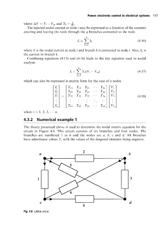
4.3.2 Numerical example 1
The theory presented above is used to determine the nodal matrix equation for the
circuit in Figure 4.8. This circuit consists of six branches and four nodes. The
branches are numbered 1 to 6 and the nodes are a, b, c and d. All branches
have admittance values Y, with the values of the diagonal elements being negative.

Fig. 4.8 Lattice circuit.