Page 132 - Power Electronic Control in Electrical Systems

//SYS21/F:/PEC/REVISES_10-11-01/075065126-CH004.3D ± 120 ± [106±152/47] 17.11.2001 9:54AM

120 Power flows in compensation and control studies

large networks which are fully interconnected and therefore have a low degree
of sparsity. In such cases there is no advantage gained by using sparsity techniques.
. By factorizing the nodal admittance matrix using sparsity techniques (Zollenkopf,
1970). In this case, the nodal admittance matrix is not inverted explicitly and the
resulting vector factors will contain almost the same degree of sparsity as the
original matrix. Sparsity techniques allow the solution of very large-scale networks
with minimum computational effort.
. By directly building up the impedance matrix (Brown, 1975). A set of rules exists to
form the nodal impedance matrix but they are not as simple as the rules used to
form the nodal admittance matrix. It outperforms the method of explicit inversion
in terms of calculation speed but the resulting impedance matrix is also full. This
approach is not competitive with respect to sparse factorization techniques.
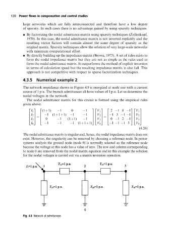
4.3.5 Numerical example 2

The network impedance shown in Figure 4.9 is energized at node one with a current
source of 1 p.u. The branch admittances all have values of 1 p.u. Let us determine the
nodal voltages in the network.
The nodal admittance matrix for this circuit is formed using the empirical rules
given above.

2 3 2 32 3 2 32 3
I 1 (1‡1) 1 0 1 V 1 2 10 1 V 1
I 2
6 7 6 1 (1‡1‡1) 1 1 76 V 2 7 6 13 1 1 76 V 2 7
ˆ
ˆ
6 7 6 76 7 6 76 7
I 3
4 5 4 0 1 (1‡1) 1 54 V 3 5 4 0 12 1 54 V 3 5
I 0 1 1 1 (1‡1‡1) V 0 1 1 13 V 0
(4:26)
The nodal admittance matrix is singular and, hence, the nodal impedance matrix does not
exist. However, the singularity can be removed by choosing a reference node. In power
systems analysis the ground node (node 0) is normally selected as the reference node
because the voltage at this node has a value of zero. The row and column corresponding
to node 0 are removed from the nodal matrix equation and in this example the solution
for the nodal voltages is carried out via a matrix inversion operation.

Fig. 4.9 Networkof admittances.