Page 130 - Power Electronic Control in Electrical Systems

//SYS21/F:/PEC/REVISES_10-11-01/075065126-CH004.3D ± 118 ± [106±152/47] 17.11.2001 9:54AM

118 Power flows in compensation and control studies

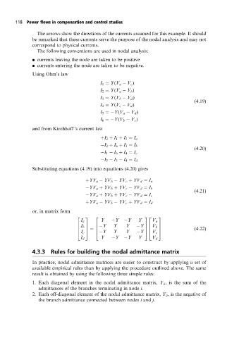
The arrows show the directions of the currents assumed for this example. It should
be remarked that these currents serve the purpose of the nodal analysis and may not
correspond to physical currents.
The following conventions are used in nodal analysis:
. currents leaving the node are taken to be positive
. currents entering the node are taken to be negative.
Using Ohm's law
I 1 ˆ Y(V a V c )
I 2 ˆ Y(V a V b )
I 3 ˆ Y(V b V d )
(4:19)
I 4 ˆ Y(V c V d )
I 5 ˆ Y(V a V d )
I 6 ˆ Y(V b V c )
and from Kirchhoff 's current law

‡I 2 ‡ I 1 ‡ I 5 ˆ I a
I 2 ‡ I 6 ‡ I 3 ˆ I b
(4:20)
I 1 I 6 ‡ I 4 ˆ I c
I 5 I 3 I 4 ˆ I d
Substituting equations (4.19) into equations (4.20) gives

‡YV a YV b YV c ‡ YV d ˆ I a
YV a ‡ YV b ‡ YV c YV d ˆ I b
(4:21)
YV a ‡ YV b ‡ YV c YV d ˆ I c
‡YV a YV b YV c ‡ YV d ˆ I d
or, in matrix form

2 3 2 32 3
I a Y Y Y Y V a
6 I b 7 6 Y Y Y Y 76 V b 7
6 7 ˆ 6 76 7 (4:22)
4 I c 5 4 Y Y Y Y 54 V c 5
I d Y Y Y Y V d

4.3.3 Rules for building the nodal admittance matrix

In practice, nodal admittance matrices are easier to construct by applying a set of
available empirical rules than by applying the procedure outlined above. The same
result is obtained by using the following three simple rules:
1. Each diagonal element in the nodal admittance matrix, Y ii , is the sum of the
admittances of the branches terminating in node i.
2. Each off-diagonal element of the nodal admittance matrix, Y ij , is the negative of
the branch admittance connected between nodes i and j.