Page 148 - Power Electronic Control in Electrical Systems

//SYS21/F:/PEC/REVISES_10-11-01/075065126-CH004.3D ± 136 ± [106±152/47] 17.11.2001 9:54AM

136 Power flows in compensation and control studies

The linearized SVC equation is given below, where the variable susceptance B SVC is
taken to be the state variable
0 0
P l y l
ˆ @Q l (4:66)
Q l 0 B SVC
@B SVC
At the end of iteration (r), the variable shunt susceptance B SVC is updated
B (r ‡ 1) ˆ B (r) ‡ B (r) (4:67)
SVC SVC SVC
4.5.3 Numerical example 5

The five-node network detailed in Section 4.4.6 is modified to include one SVC
connected at node Lake to maintain the nodal voltage magnitude at 1 p.u. Conver-
gence is obtained in four iterations to a power mismatch tolerance of e 10 12 using
an OOP Newton±Raphson power flow program (Fuerte-Esquivel et al., 1988). The
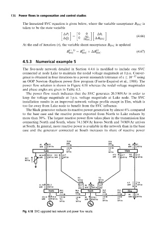
power flow solution is shown in Figure 4.18 whereas the nodal voltage magnitudes
and phase angles are given in Table 4.5.
The power flow result indicates that the SVC generates 20.5 MVAr in order to
keep the voltage magnitude at 1 p.u. voltage magnitude at Lake node. The SVC
installation results in an improved network voltage profile except in Elm, which is
too far away from Lake node to benefit from the SVC influence.
The Slack generator reduces its reactive power generation by almost 6% compared
to the base case and the reactive power exported from North to Lake reduces by
more than 30%. The largest reactive power flow takes place in the transmission line
connecting North and South, where 74.1 MVAr leaves North and 74 MVAr arrives
at South. In general, more reactive power is available in the network than in the base
case and the generator connected at South increases its share of reactive power

Fig. 4.18 SVC upgraded test networkand power flow results.