Page 59 - Power Electronic Control in Electrical Systems

//SYS21/F:/PEC/REVISES_10-11-01/075065126-CH002.3D ± 49 ± [31±81/51] 17.11.2001 9:49AM

Power electronic control in electrical systems 49

Some of the generators in a large system may be operated at light load in a state of
readiness or `spinning reserve', in case the system load increases suddenly by a large
amount. This can happen, for example, at the end of television transmissions when
the number of viewers is exceptionally high.

2.8.1 Relationships between power, reactive power, voltage
levels and load angle

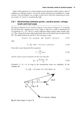
The phasor diagram for the system in Figure 2.16 is shown in Figure 2.17, assuming
that the load has a lagging power factor angle f. The line or cable is represented by
its impedance R s ‡ jX s , and R s is again neglected (being usually much smaller than
X s ). The voltage drop across the transmission line is jX s I, which leads the phasor I by
90 . The angle between E s and E r is the load angle, d and

E s cos d ˆ E r ‡ X s I sin f and E s sin d ˆ X s I cos f (2:17)

Also
P ‡ jQ ˆ E r I ˆ E r I cos f ‡ jE r I sin f (2:18)

From this we get the power flow equation

E s E r
P ˆ sin d (2:19)
X s
and the reactive power equation for the receiving end
E s cos d E r
Q r ˆ E r (2:20)
X s
Evidently P ˆ P s ˆ P r as long as the transmission losses are negligible. At the
sending end,
P s ‡ jQ s ˆ E s I cos(f ‡ d) ‡ jE s I sin(f ‡ d) (2:21)

Fig. 2.17 Phasor diagram for Figure 2.16.