Page 56 - Power Electronic Control in Electrical Systems

//SYS21/F:/PEC/REVISES_10-11-01/075065126-CH002.3D ± 46 ± [31±81/51] 17.11.2001 9:49AM

46 Power systems engineering ± fundamental concepts

I γ

E jX ss
I
I s
∆V
R s I s
V

I
Load
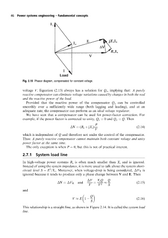
Fig. 2.15 Phasor diagram, compensated for constant voltage.

voltage V. Equation (2.13) always has a solution for Q s , implying that: A purely
reactive compensator can eliminate voltage variations caused by changes in both the real
and the reactive power of the load.
Provided that the reactive power of the compensator Q g can be controlled
smoothly over a sufficiently wide range (both lagging and leading), and at an
adequate rate, the compensator can perform as an ideal voltage regulator.
We have seen that a compensator can be used for power-factor correction. For
example, if the power factor is corrected to unity, Q s ˆ 0and Q g ˆ Q. Then
P
V ˆ (R s ‡ jX s ) (2:14)
V
which is independent of Q and therefore not under the control of the compensator.
Thus: A purely reactive compensator cannot maintain both constant voltage and unity
power factor at the same time.
The only exception is when P ˆ 0, but this is not of practical interest.
2.7.1 System load line

In high-voltage power systems R s is often much smaller than X s and is ignored.
Instead of using the system impedance, it is more usual to talkabout the system short-
2
circuit level S ˆ E /X s . Moreover, when voltage-drop is being considered, V X is
ignored because it tends to produce only a phase change between V and E. Then
V X s Q Q
V ˆ V R and ˆ (2:15)
V V 2 S
and

Q
V E 1 (2:16)
S
This relationship is a straight line, as shown in Figure 2.14. It is called the system load
line.