Page 55 - Power Electronic Control in Electrical Systems

//SYS21/F:/PEC/REVISES_10-11-01/075065126-CH002.3D ± 45 ± [31±81/51] 17.11.2001 9:49AM

Power electronic control in electrical systems 45

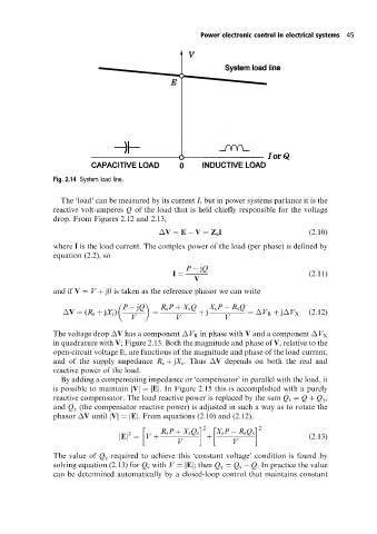
Fig. 2.14 System load line.

The `load' can be measured by its current I, but in power systems parlance it is the
reactive volt-amperes Q of the load that is held chiefly responsible for the voltage
drop. From Figures 2.12 and 2.13,
V ˆ E V ˆ Z s I (2:10)
where I is the load current. The complex power of the load (per phase) is defined by
equation (2.2), so
P jQ
I ˆ (2:11)
V
and if V ˆ V ‡ j0 is taken as the reference phasor we can write
P jQ R s P ‡ X s Q X s P R s Q

V ˆ (R s ‡ jX s ) ˆ ‡ j ˆ V R ‡ j V X (2:12)
V V V
The voltage drop V has a component V R in phase with V and a component V X
in quadrature with V; Figure 2.13. Both the magnitude and phase of V, relative to the
open-circuit voltage E, are functions of the magnitude and phase of the load current,
and of the supply impedance R s ‡ jX s . Thus V depends on both the real and
reactive power of the load.
By adding a compensating impedance or `compensator' in parallel with the load, it
is possible to maintain jVjˆjEj: In Figure 2.15 this is accomplished with a purely
reactive compensator. The load reactive power is replaced by the sum Q s ˆ Q ‡ Q g ,
and Q g (the compensator reactive power) is adjusted in such a way as to rotate the
phasor V until jVjˆ jEj. From equations (2.10) and (2.12),
2 2
2 R s P ‡ X s Q s X s P R s Q s
jEj ˆ V ‡ ‡ (2:13)
V V
The value of Q g required to achieve this `constant voltage' condition is found by
solving equation (2.13) for Q s with V ˆjEj; then Q g ˆ Q s Q. In practice the value
can be determined automatically by a closed-loop control that maintains constant