Page 126 - Practical Control Engineering a Guide for Engineers, Managers, and Practitioners

A New Do11ain and More Process Models 101

to 1
.. . .
(I)
"'0
.a
:.= tOO
Q.. ''
~
to-I
to-2 to-I to 0
too
- 0
~
(I)
U) -100 Dead time= 8
cu
f
-200
-300
to-2 to 0
Radian frequency
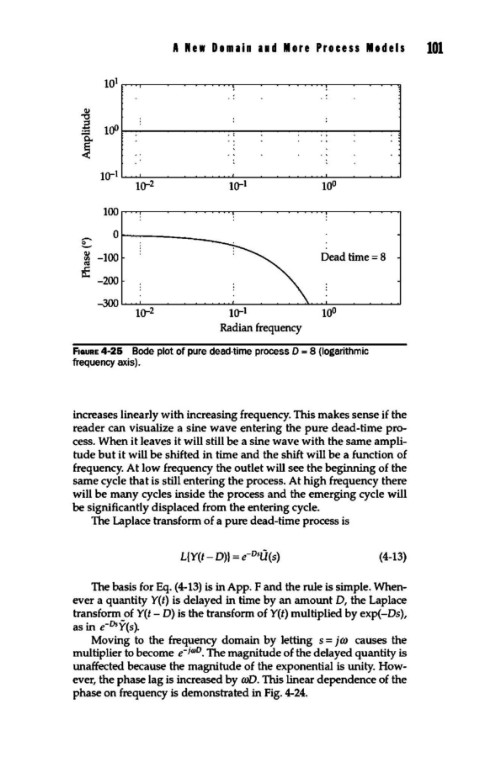
F1GURE4-26 Bode plot of pure dead-time process D = 8 (logarithmic
frequency axis).

increases linearly with increasing frequency. This makes sense if the
reader can visualize a sine wave entering the pure dead-time pro-
cess. When it leaves it will still be a sine wave with the same ampli-
tude but it will be shifted in time and the shift will be a function of
frequency. At low frequency the outlet will see the beginning of the
same cycle that is still entering the process. At high frequency there
will be many cycles inside the process and the emerging cycle will
be significantly displaced from the entering cycle.
The Laplace transform of a pure dead-time process is

L{Y(t- D)J = e-Dszi(s) (4-t3)

The basis for Eq. (4-t3) is in App. F and the rule is simple. When-
ever a quantity Y(t) is delayed in time by an amount D, the Laplace
transform of Y(t- D) is the transform of Y(t) multiplied by exp(-Ds),
as in e-DsY(s).
Moving to the frequency domain by letting s = jm causes the
multiplier to become e-iOJD. The magnitude of the delayed quantity is
unaffected because the magnitude of the exponential is unity. How-
ever, the phase lag is increased by roD. This linear dependence of the
phase on frequency is demonstrated in Fig. 4-24.