Page 164 - Practical Control Engineering a Guide for Engineers, Managers, and Practitioners

Matrices and Higher-Order Process Models 139

.........
~~ 0~------~--~----,
...
~
5'~ -50
.,~
...
-~ -100
~+
.a c -150
·~ -200 L-n-4____.____.__. ............... ........,____.___._ .......................... ___.__._ ........................... ___. ............................ ..........~
~ 1u . 10-3 10-2 10-1 100
0.---------==~~~.-~--~~------~
.........
~~- -100
... ~~
~ ...
C)'~ -200
-+
M c -30o
..c
p..
~o~~~~~--~~~~--~~~~~~~~
1o-4 1~ 1~ 1~ ~
Frequency
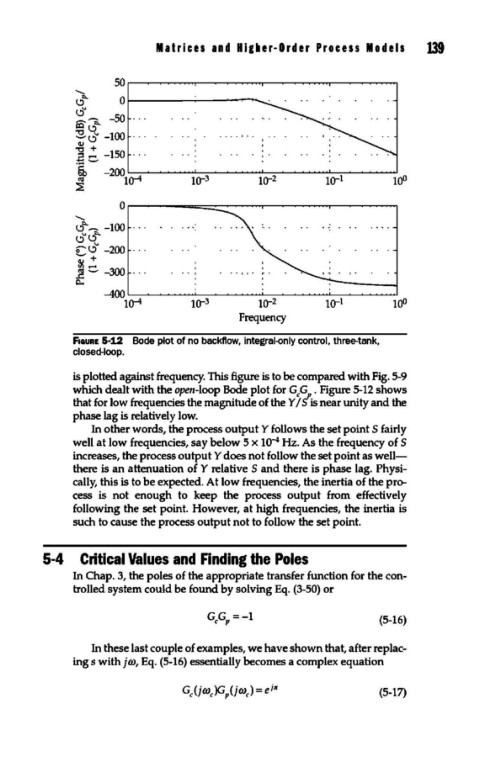
F1aURE 5-12 Bode plot of no backflow, integral-only control, three-tank,
closed-loop.
is plotted against frequency. This figure is to be compared with Fig. 5-9
which dealt with the open-loop Bode plot for G,G,. Figure 5-12 shows
that for low frequencies the magnitude of the Y IS is near unity and the
phase lag is relatively low.
In other words, the process output Y follows the set point S fairly
well at low frequencies, say below 5 x 1o-' Hz. As the frequency of S
increases, the process output Y does not follow the set point as well-
there is an attenuation of Y relative S and there is phase lag. Physi-
cally, this is to be expected. At low frequencies, the inertia of the pro-
cess is not enough to keep the process output from effectively
following the set point. However, at high frequencies, the inertia is
such to cause the process output not to follow the set point.

5-4 Critical Values and Finding the Poles
In Chap. 3, the poles of the appropriate transfer function for the con-
trolled system could be found by solving Eq. (3-50) or

(5-16)

In these last couple of examples, we have shown that, after replac-
ing s with jm, Eq. (5-16) essentially becomes a complex equation

(5-17)