Page 205 - Practical Design Ships and Floating Structures

180

Extreme Value (PEV) at possibility level a (risk parameter) can be determined by (Bhattacharyya,
1978; Ochi, 1981)

for E S 0.9 (2)

.
,
Ts
in which N is the number of observations (or cycles), N = (60) - + J‘:2 E and rq is the time
4n JG-
length of wave data, unit of time in hours. When a=l, xPE,,=xeJ,,=, represents the value that may be
exceeded once out of N observations. a (I 1) is chosen at the designer’s discretion, depending on the
condition of application. Figure 6 indicates the dependency of E vs. spectral peak periods in a WSD. In
this figure, the range of E of the stress responses is mostly between 0.25 and 0.40. It is found that E can
easily be close to 0.4, and an error at the 5% to 10% level could be introduced for N if E is ignored. So
it is suggested that a correction for E should always be used.
When the short-term approach is used, a design wave spectrum of the extreme storm condition is
usually provided with a long-term extreme value of H, and related T. Ochi’s (1981) results indicate
that the probability density function of (H, takes a bivariate log-normal distribution. A commonly
used approach is to determine the long-term extreme of H, first, and then the T is obtained with the
conditional probability distribution p(7lHS) or a simple formula between H, and T based on the wave
steepness.
The long-term PEV of H, with different return periods is listed in Table 1, in which H, is calculated by
applying the long-term extreme approach discussed in the next section. To determine the extreme wave
environment (two parameter wave spectra in this example) used in the short-term approach, Tp is
required. Table 2 lists the peak periods associated with H,. The values of Tp are calculated by using
p(71Hs) at confidence levels 0.5,0.75,0.85, and 0.95, separately (Ochi, 1978). Each H, and the related
Tp form a wave spectral family, which is used to determine the response spectrum, and finally the
short-term extreme values.

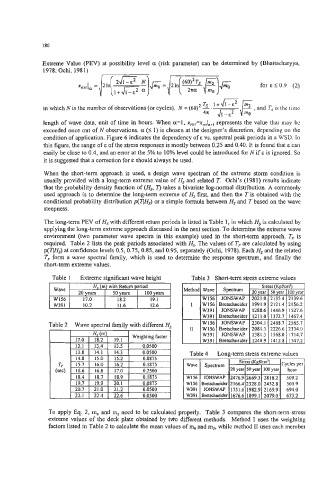
Table 1 Extreme significant wave height Table 3 Short-term stress extreme values
Hs (m) with Return period
wave 20years I 50years I 100 years
W156 17.0 I 18.2 I 12.6 I I I 1 W1561 JONSWAP 2021.0 12135.4 12139.6
19.1
.. .
I W391 I 10.2 I 11.6 1
W391 Bretschneider 121 1.0 1372.7 1467.4
Table 2 Wave spectral family with different H, W156 JONSWAP 2304.1 2468.7 2565.7
, ~~ I1 W156 Bretschneider 2081.3 2226.6 2334.0
Weighting factor W391 JONSWAP 1381.3 1568.0 1714.7
W391 Bretschneider 1248.9 1412.8 1547.2
13.4 0.0500
0.0500 Table 4 Long-term stress extreme values
n nx75

W156 JONSWAP 2416.9 2669.3 2818.2 509.2
WIS6 Bretschneider 2166.4 2328.0 2452.8 500.9
1751.6 1982.9 2169.9 694.0
1676.6 1899.1 2079.0 673.2

To apply Eq. 2, m, and m2 need to be calculated properly. Table 3 compares the short-term stress
extreme values of the deck plate obtained by mo different methods. Method I uses the weighting
factors listed in Table 2 to cdculate the mean values of m, and m,, while method I1 uses each member