Page 206 - Practical Design Ships and Floating Structures

I81

of the spectral family in Table 2, and takes the maximum. The extreme values provided by the latter
are up to 16% larger than those by the former method. This is understandable because the sample size
(or exposure time) for the latter is relatively larger. In this example, extreme values for H, with risk
parameter a = 1 are directly applied. Obviously, the final extreme values of responses are dependent
on the designer's discretion and choice of Ifs

4.2 Long-term Extreme Approach
To predict a long-term extreme value, a long-term initial cumulative probability distribution function
P(x) of responses is required. Although function P(x) cannot be predicted explicitly due to the
complications of the responses in various sea states, it can be built up approximately through
accumulations of short-term statistical analyses. Generally, P(x) can be assumed to be in the form of
P(x) = 1 - exp[-q(x)] (q(420) (3)
In practice, a Weibull distribution or log-normal distribution is commonly used for P(x). In this paper a
generalized fonn suggested by Ochi (1981) is used to achieve higher accuracy in the curve fitting. i.e.,
q(x) = cxm exp(-pxk), in which c, m, p, and k are four constant parameters to be determined by
nonlinear least-squared fitting. Once the mathematical expression of P(x) in Eq. 3 is obtained, the
long-term PEV can be determined by

Here a is the possibility level as in Eq. 2. Here N is the number of observations or cycles related to the
return period. In the design of offshore structures, a return period of IO0 years is widely used for
estimating the long-term extreme values. When the WSD is applied, the P(x) above can be obtained by
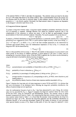
using the definition of probability density function of maxima
1 "ijkl p<wij ) Pr(Qk Pr(A1 )pgk/ (x)
p(x) = UkJ (5)
c "ijkl pr(w& Pr(a k ) pr(Al)
WJ
where
Pr(w,): normalized joint wave probability of (HdzJ,mJ) or cell w# in WSD, CPr(wii) = 1.
iJ
Pr(a,): probability of wave in direction a, CPr(ak) = 1.
k
Pr(A,): probability (or percentage) of loading pattern A, during service, XPr(Al) = 1.
I
n,,,: average number of responses in T, corresponding to cell wil of WSD, wave direction ak and
loading pattern A,.
p,&): the probability density function of short-term response maxima associated with n,,,.
Figure 7 displays the long-term p(x) of stress responses to waves W156 and W391. It is obvious that
the wave environment is the dominant factor affecting the long-term probability distribution; the
effects of spectral shape are not significant.
Afier the mathematical formula of q(x) in Eq. 3 has been determined by curve fitting, the extreme
value can be calculated by Eq. 4. Figure 8 compares the long-term extreme values for wave zones
W156 and W391 using the JONSWAP and Bretschneider spectra. The extreme values of stress
dynamic components are listed in Table 4. By comparing the long-term extreme values to those short-
term extreme values listed in Table 3, it is found that the extreme values provided by the long-term
approach are larger up to 9%. Because the long-term approach uses the probability distribution of
responses directly, it can avoid the uncertainty caused by the choice of extreme If, and associated
wave spectral family (a series of Tp). Based on this point of view, the long-term approach is more