Page 243 - Process Equipment and Plant Design Principles and Practices by Subhabrata Ray Gargi Das

9.3 Representation of equilibrium 243

(F) (G) q max
60°C 50°C 40°C
(Partial pressure of solute over liquid) pi 30°C Adsorbate loading q

x Adsorbate conc. in solution, c
(mol. fraction of solute gas in liquid)

(H) B

20 80
40 60
Plait point
60 40
80 20
Tie lines
A S
20 40 60 80
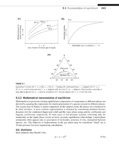
FIGURE 9.1
Equilibrium Curves (A) T x y (B) x y (C) X Y along with corresponding x y diagram (D) P x y
(E) H x y and corresponding T x y diagram with tie lines (F) p i x diagram (Hydrocarbon solubility in
poly-alkene glycol) (G) q c plot for adsorption (H) Ternary diagram for L L E with tie lines.

9.3.2 Mathematical representation of equilibrium
Mathematical expressions relating equilibrium composition of components in different phases are
derived by equating the expressions for chemical potential of a species present in different phases.
The system may be binary or multi-component. In the simplest form, the phases are considered to
be ideal mixtures. A more realistic representation is obtained by considering nonideal thermo-
dynamics for the condensed (liquid and solid) and the vapor phase using activity coefficients and
fugacity coefficients, respectively. In most cases of low-pressure systems, correcting only for
nonideality in the liquid phase results in fairly accurate equilibrium relationships. Liquid phase
nonideality often appears due to association of molecules, presence of ions, interaction between
species, etc. The behavior of hydrocarbons in the gas phase may be considered “ideal” up to
10 atm pressure for most engineering calculations.

VLE: Distillation
Ideal solutions obey Raoult’s law:

p i ¼ x i p sat (9.1a)
i