Page 245 - Process Equipment and Plant Design Principles and Practices by Subhabrata Ray Gargi Das

Solubility: absorption and stripping
Solubility data of a gaseous component in the liquid phase needs to be known for absorber and stripper
design. Equilibrium solubility of components of a gas mixture over a liquid is often expressed in terms
of partial pressure of the component (Table 9.3). An ideal dilute solution is described by Henry’s law:
p i ¼ H i x i , for components in minute quantities (x i /0). H i , the Henry’s law constant for
component i depends on temperature but is relatively independent of system pressure at moderate
pressure levels. x i 0:1 is considered as the upper limit for applicability of Henry’s law within en-
gineering accuracy.
The solubility of gas decreases with increasing temperature, and hence, the equilibrium (solubility)
curves are steeper at higher temperatures, as is evident from Fig. 9.1F. Gas solubility increases with
pressure, and it is possible to produce any gas concentration in the liquid by applying sufficient
pressure as long as the liquefied form of the gas is completely soluble in the liquid. Solubility of a gas
is affected by presence of other gases in the system and also by the presence of nonvolatile solute.
The aforementioned relationships are applicable to nonreactive systems only and cannot be used
for systems where the absorbed gas reacts with the solvent.
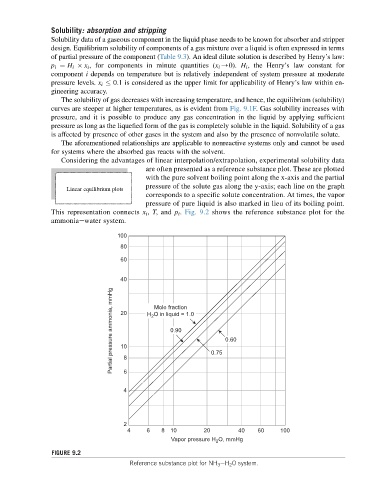
Considering the advantages of linear interpolation/extrapolation, experimental solubility data
are often presented as a reference substance plot. These are plotted
with the pure solvent boiling point along the x-axis and the partial
pressure of the solute gas along the y-axis; each line on the graph
Linear equilibrium plots
corresponds to a specific solute concentration. At times, the vapor
pressure of pure liquid is also marked in lieu of its boiling point.
This representation connects x i , T,and p i . Fig. 9.2 shows the reference substance plot for the
ammoniaewater system.
100
80
60

40
Partial pressure ammonia, mmHg 20 8 H O in liquid = 1.0 0.75 0.60

Mole fraction
2

0.90

10

4 6

2
4 6 8 10 20 40 60 100
O, mmHg
Vapor pressure H 2
FIGURE 9.2
Reference substance plot for NH 3 eH 2 O system.