Page 244 - Process Equipment and Plant Design Principles and Practices by Subhabrata Ray Gargi Das

244 Chapter 9 Phase equilibria

where p i is the equilibrium partial pressure of component i present in solution, x i is the mole fraction in
sat
the liquid phase, and p i is the vapor pressure of the pure component at the same temperature.
Raoult’s law is valid for chemically similar liquids or for components in large excess, i.e., as x i / 1
the prediction accuracy improves.
Inclusion of activity coefficient (g ) accounts for nonideality of the liquid phase and modifies the
i
expression as:
sat
p i ¼ g x i p (9.1b)
i i
The equilibrium vapor-phase mole fraction (y ) for both phases ideal is

i
sat
y ¼ p i =P ¼ x i p =P (9.2a)

i i
and for nonideality in the liquid phase is
sat
y ¼ p i =P ¼ g x i p =P (9.2b)

i i i
where P is the total system pressure.
Data on activity coefficients/equations to evaluate the same can be obtained from any standard
textbook on phase equilibrium thermodynamics.
Equilibrium data are also presented in the form of equilibrium constant K i for component i.It is
termed distribution coefficient and is commonly used in case of hydrocarbon systems.
K i ¼ y =x i (9.3)

i
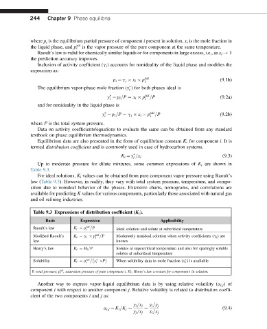
Up to moderate pressure for dilute mixtures, some common expressions of K i are shown in
Table 9.3.
For ideal solutions, K i values can be obtained from pure component vapor pressure using Raoult’s
law (Table 9.3). However, in reality, they vary with total system pressure, temperature, and compo-
sition due to nonideal behavior of the phases. Extensive charts, nomograms, and correlations are
available for predicting K values for various components, particularly those associated with natural gas
and oil refining industries.

Table 9.3 Expressions of distribution coefficient (K i ).
Basis Expression Applicability
Raoult’s law K i ¼ p sat P Ideal solution and solute at subcritical temperature
i
Modified Raoult’s K i ¼ g i p sat P Moderately nonideal solution when activity coefficients (g i ) are
i
law known
Henry’s law K i ¼ H i =P Solutes at supercritical temperature and also for sparingly soluble
solutes at subcritical temperature
Solubility K i ¼ p sat x P When solubility data in mole fraction (x ) is available

i
i
i
sat
P, total pressure;p i , saturation pressure of pure component i;H i , Henry’s law constant for component i in solution.
Another way to express vapor-liquid equilibrium data is by using relative volatility (a i;j )of
component i with respect to another component j. Relative volatility is related to distribution coeffi-
cient of the two components i and j as:
y i =x i y i =y j
(9.4)
a i;j ¼ K i =K j ¼ ¼
y j =x j x i =x j