Page 200 - Radar Technology Encyclopedia

filter, Kalman(-Bucy) filter, linear 190

(2) The measurement model has to be specified. For the sources move back and forth, creating a spectrum that is sym-
Kalman filter this would have the form metrical about zero doppler. DKB
Kalmus, H. P., “Doppler Wave Recognition with High Clutter Rejection,”
+
=
×
d()
y n () H x n () y n IEEE Trans. AES-3, no. 6 (Eastcon Suppl.), Nov. 1967, pp. 334–339;
s
Skolnik (1980), p. 497.
where y n ()
is the vector of measured coordinates at tn, x n ()
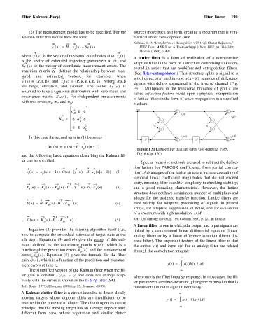
s A lattice filter is a form of realization of a nonrecursive
is the vector of estimated trajectory parameters at tn, and
adaptive filter in the form of a structure comprising links con-
is the vector of coordinate measurement errors. The
d y n ()
nected in series that are nonbifurcated extrapolation filters.
transition matrix H defines the relationship between mea-
(See filter-extrapolator.) This structure splits a signal to a
sured and estimated vectors; for example, when
samples of difference
and inverse e n –
· · · set of direct e n () ( N )
y n () ( R eb,, ) s = RR eebb, ,,, ,) signals with delays augmented in the inverse channel (Fig.
and x n () (
=
, where R,e,b
are range, elevation, and azimuth. The vector d y n ()
is
F31). Multipliers in the transverse branches of grid k are
assumed to have a Gaussian distribution with zero mean and
called reflection factors based upon a physical interpretation
covariance matrix Km n ()
. For independent measurements
of lattice filters in the form of wave propagation in a stratified
with rms errors s, s , and s :
r e b medium.
2 y(n)
s 00 S S
R e (n)
1 e (n)
K = 2 N
m 0 s b 0
2 k 1 k N
0 0 s
e
~ ~ e (n-N)
In this case the second term in (1) becomes e (n-1) N
1
z -1 S z -1 S
Dy n () y n () Hx nn ––= × ( 1 )
p Figure F31 Lattice filter diagram (after Gol’denberg, 1985,
Fig. 6.6, p. 170).
and the following basic equations describing the Kalman fil-
ter can be specified: Special recursive methods are used to subtract the deflec-
tion factors (or PARCOR coefficients, from partial correla-
[
–
×
×
(
+
x n () x nn –= p ( 1 ) Gn () y n () Hx nn – 1 )] (2) tion). Advantages of the lattice structure include cascading of
s
p
identical links; coefficient magnitudes that do not exceed
unity, ensuring filter stability; simplicity in checking stability;
T – 1
K n () K n () K n ()H × n × × and a good rounding characteristic. However, the lattice
S ()HK n () (3)
=
×
–
s p p p
structure does not have a minimum number of multipliers and
adders for the assigned transfer function. Lattice filters are
T – 1
×
×
=
Sn () HK n ()H K × n () (4) used widely for adaptive processing of signals in phased
p m
arrays, for adaptive suppression of noise, and for evaluation
of a spectrum with high resolution. IAM
T – 1
Gn () K n ()H K × n () (5) Ref.: Gol’denberg (1985), p. 169; Cowan (1985), p. 123, in Russian.
×
=
s m
A linear filter is one in which the output and input signals are
Equation (2) provides the filtering algorithm itself (i.e., linked by a conventional linear differential equation (linear
how to compute the smoothed estimate of target state at the analog filter) or by a linear difference equation (linear dis-
nth step). Equations (3) and (4) give the errors of this esti- crete filter). The important feature of the linear filter is that
, which is a
mate, defined by the covariance matrix K n ()
s the output y(t) and input x(t) for an analog filter are related
and the measurement
function of the prediction errors K n ()
p through the convolution integral:
. Equation (5) gives the formula for the filter
n
errors K ()
m ¥
, which is a function of the prediction and measure-
gain Gn ()
d
ment errors at time t . yt () = ò xt () ht t,( ) t
n
The simplified version of the Kalman filter when the fil- – ¥
ter gain is constant, Gn () G and does not change adap-
=
where h(t) is the filter impulse response. In most cases the fil-
tively with the errors is known as the a-b(-g) filter. SAL
ter parameters are time-invariant, giving the expression that is
Ref.: Bozic (1979); Blackman (1986), p. 25; Brammer (1989). fundamental in radar signal filter theory:
A Kalmus clutter filter is a circuit intended to detect slowly ¥
moving targets whose doppler shifts are insufficient to be
d
(
yt () = ò xt – t ) h t()t
resolved in the presence of clutter. The circuit operates on the
– ¥
principle that the moving target has an average doppler shift
different from zero, where vegetation and similar clutter