Page 199 - Radar Technology Encyclopedia

189 filter, high-pass filter, Kalman(-Bucy)

|H(f)| Spectral density
Insertion loss
Noise Clutter
1.0 Signal
Frequency
f - f r f f + f r
0 0 0
Passband (a) Input signal + interference spectrum
Spectral density
Transition band
Attenuation level
f
0
Frequency
0
0
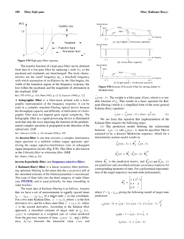
Figure F29 High-pass filter response. f - f r f 0 f + f r
(b) Inverse filter response
The transfer function of a high-pass filter can be obtained Spectral density
from that of a low-pass filter by replacing s with 1/s, so the Noise
passband and stopbands are interchanged. The main charac- Signal
teristics are the cutoff frequency w , a threshold frequency Frequency
c
with which attenuation of oscillations by the filter begins, the f - f r f 0 f + f r
0
0
(c) Output signal + interference spectrum
width of the transition region of the frequency response, the
loss within the passband, and the magnitude of attenuation in Figure F30 Inverse (Urkowitz) filter for strong clutter in
thermal noise.
the stopband. IAM
Ref.: ITT (1975), p. 10.8; Fink (1982), p. 12.32; Sazonov (1988), p. 122. ˆ
. The weight is a filter gain, G(an), which is a vari-
(
x nn – 1 )
s
A holographic filter is a filter-mask printed with a holo- able function of t . This results in a basic equation for Kal-
n
graphic representation of the frequency response. It can be man filtering (which is a simplified form of the more general
used in a complex matched filtering optical device because Kalman-Bucy equation):
the throughput capacity and difficulty of fabrication of a holo- ˆ
+
×
graphic filter does not depend upon signal complexity. The x n () x nn –= p ( 1 ) Gn () D y n () (1)
s
holographic filter in a signal-processing device is illuminated We see from this equation that implementation of the
such that only the wave depicting the function of the predeter- Kalman filter requires the following steps:
mined complex spectrum is propagated in the direction of the (1) The prediction model defining the relationship
ˆ
ˆ
optical axis. IAM between x n – 1 ) and x nn – 1 )
must be specified. This is
(
(
s p
Ref.: Dulevich (1978), p. 165; Zmuda (1994) p. 399. assumed to be a discrete Markovian sequence, which for a
An inverse filter is one that converts a complex interference deterministic motion model results in
input spectrum to a uniform (white) output spectrum, opti-
x nn – 1 ) = F x n – 1 )
(
(
×
mizing the output signal-to-interference ratio of subsequent p p s
signal integration circuits (Fig. F30). This filter is also known
as the Urkowitz filter or whitening filter. DKB T
K n () = p F K n – 1 ) F
×
(
×
p
p
s
Ref.: Barton (1988), p. 236.
(
inverse hyperbolic filter (see frequency-selective filter). where F p is the prediction matrix, and K n () and K n – 1 )
s
p
are prediction and smoothed estimate covariance matrices for
A Kalman(-Bucy) filter is a linear recursive filter perform-
corresponding moments of time. For a polynomial representa-
ing optimum filtering in the sense that the a posteriori pdf of
tion of the target trajectory (second-order polynomial),
the smoothed estimate of the filtered parameter is maximized.
This type of filter falls into the third category of radar filters 2
1 TT ¤ 2
(see FILTER) and is used primarily for data smoothing in F =
radar trackers. p 01 T
The main idea of Kalman filtering is as follows. Assume 00 1
that we have a set of measurements at equally spaced times where T = t - t n-1 , giving the following model of target state
n
t , ... , t n-1 , ... , t , t n+1 of a target state x in one coordinate. prediction:
1
n
·
, where is the first
For a two-state Kalman filter, x = ( xx , ) x · 2
· ·· ˆ · ˆ ·· ˆ T
, where
,,
derivative of x, and for a three-state filter x = ( xx x ) x nn – 1 ) x n – 1 ) x s n – 1 )T + x s n – 1 )-----
×
(
×
(
+
=
(
(
·· p s 2
x is the second derivative. According to the Kalman filter
approach, a smoothed estimate of target state at t , (i.e.,
n
ˆ · ˆ · ·· ˆ
) is computed as a weighted sum of values predicted
×
+
(
x n () x p nn – 1 = x s n – 1 ) x s T
s
ˆ
, and a differ-
(
from the previous moment of time, x nn – 1 )
s
·· ˆ
··
between the measured value y n ()
ence Dy n () and x p nn – 1 ) x s n – 1 )
(
(
=