Page 91 - Radar Technology Encyclopedia

clutter (amplitude) distribution clutter (amplitude) distribution 81

normal pdf appears as a normal distribution on a decibel
Table C1
scale, and when the standard distribution s is set to 4 dB, this Typical PDFs Used to Describe Clutter Amplitudes
y
distribution gives a close match to the Rayleigh for ampli-
tudes near or above the median. The Weibull family of pdfs
Distribution and analytical form Scattering conditions
have shapes such that the ath root of the amplitude is Ray-
leigh distributed, and hence their breadth increases in propor- Gaussian In-phase or quadrature volt-
tion to the parameter a, while the density decreases with this 1 – ( x – x ) age components of many
2
scattering centers with ran-
parameter. Another distribution used to describe clutter is the Wx () ----------------- exp= 2ps x ---------------------- dx dom phase
2
2s
K-distribution, which may be thought of as the pdf of a Gaus- x
sian vector whose variance is modulated by a gamma distri-
Rayleigh (voltage) Many scattering centers with
bution (Farina, et al., 1995). This type of distribution is useful random phase
æ 2 ö
x –
in describing clutter such as waves at sea, rolling terrain, or Wx () ------ exp= x ç ---------- ÷ dp
2 ç 2 ÷
rain cells, observed with radar resolution capable of separat- s x è 2s ø
x
ing regions of different mean level.
The large peak amplitudes encountered in non-Rayleigh Exponential (power) Many scattering centers with
clutter make it difficult to control false alarms with conven- Wp () --- exp= 1 æ – p ö random phase
------ dp
p è p ø
tional CFAR techniques. Two-parameter CFAR, in which the
spread of the pdf is measured and used to set the threshold
Rician (voltage) Constant-amplitude domi-
higher above the mean than with Rayleigh clutter, causes nant scatterer plus many
æ 2 d 2 ö æ ö
x +
(
)
greater target suppression, which can be expressed in the Wx () ------ exp= x ç – -------------------------- ÷ xd ÷ smaller with random phase
ç
------ dx
I
2 ç 2 ÷ 0ç 2 ÷
è
radar equation as a clutter distribution loss (see LOSS). Clut- s x è 2s x ø s ø
x
ter maps, which permit setting a separate threshold for each
resolution cell, can be used to restrict target suppression to the Weibull (power) Scattering from a collection
of several size classes of
few cells actually containing strong clutter. The ability to p 1 a ¤ æ p 1 a ¤ ö scatterers
Wp () --------------- exp= – ç --------------- ÷ dp
detect targets between such strong clutter cells has been aap è a ø
termed interclutter visibility (Barton and Shrader, 1969). Typ-
Log-normal Scattering from a collection
ical pdfs used to describe clutter amplitudes are given in of scatterers of different
2
Table C1 and illustrated in Figs. C18 through C25. DKB 1 ( y – y ) sizes, including a small num-
Wy () ----------------- exp= – ------------------- dy ber of large scatterers
2ps 2
Ref.: Barton, D. K., and Shrader, W. W., “Interclutter Visibility in MTI Sys- y 2s
y
tems,” IEEE Eascon Record, 1969, pp. 294–297; Schleher (1991), p. 19;
Currie (1992), pp. 14–27; Farina, A., et al., “Coherent Radar Detection
x is a voltage, p is a power, y is a decibel value, s x and s y are the standard devia-
2
of Targets against a Combination of K-Distributed and Gaussian Clut- tions, x, p, and y are the mean values, m is the ratio of power of the steady compo-
ter,” IEEE Radar-95, May 8-11, 1995, pp. 83–88. nent to the average of the random component, a is the Weibull spread parameter,
and a is the Weibull power parameter.
0.1
s y = 4 dB
0.4
Probability density per dB 0.06 s = 8 dB Probability density 0.2
0.08
a = 1
0.3
y
0.1
0.04
0
a = 2
1
0
3
2
Voltage in units of standard deviation
0.02
Figure C19 Gaussian distribution. 1 2 3
0.7
0
30 20 10 0 10 20
0.6
Value in dB relative to median 0.5
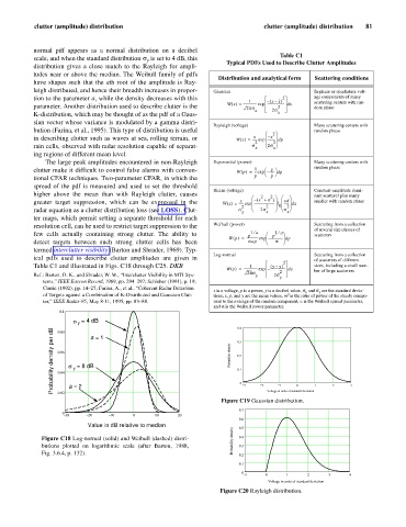
Figure C18 Log-normal (solid) and Weibull (dashed) distri- Probability density 0.4
butions plotted on logarithmic scale (after Barton, 1988, 0.3
Fig. 3.6.4, p. 132). 0.2
0.1
0
1 0 1 2 3 4
Voltage in units of standard deviation
Figure C20 Rayleigh distribution.