Page 90 - Radar Technology Encyclopedia

80 clutter, cloud clutter (amplitude) distribution

should be defined such that the number of statistically inde-
50
pendent clutter samples n obtained within a given observa-
c
60
tion time t will be
o
70
t ---- o c
n =
1 +
Reflectivity in dB(m 2 /m 3 ) 100 90 l = 3.2 mm l l = 2 cm l = 5.4 cm This relationship corresponds to t = 1/b , where b is the
c
80
t
= 8.6 mm
n
c
n
noise bandwidth of the clutter spectrum. A similar relation-
= 3.2 cm
110
ship applies to samples available over an observation fre-
l
= 10 cm
120
l
is f :
130
c
l = 23 cm quency interval Df when the frequency correlation interval
Df
140 -----
n = 1 +
c f
150 c
The correlation distance interval is similarly defined in
160
0.01 0.1 1 10
space and is often controlled by the resolution of the radar,
Cloud density in g/m 3
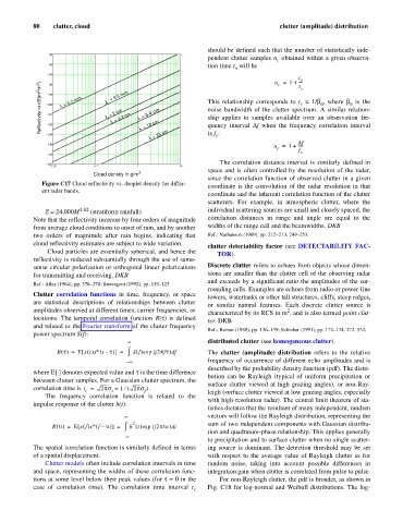
since the correlation function of observed clutter in a given
Figure C17 Cloud reflectivity vs. droplet density for differ-
coordinate is the convolution of the radar resolution in that
ent radar bands.
coordinate and the inherent correlation function of the clutter
scatterers. For example, in atmospheric clutter, where the
Z = 24,000M 1.82 (stratiform rainfall). individual scattering sources are small and closely spaced, the
Note that the reflectivity increase by four orders of magnitude correlation distances in range and angle are equal to the
from average cloud conditions to onset of rain, and by another widths of the range cell and the beamwidths. DKB
two orders of magnitude after rain begins, indicating that Ref.: Nathanson (1969), pp. 212–213, 249–253.
cloud reflectivity estimates are subject to wide variation.
clutter detectability factor (see DETECTABILITY FAC-
Cloud particles are essentially spherical, and hence the
TOR).
reflectivity is reduced substantially through the use of same-
sense circular polarization or orthogonal linear polarizations Discrete clutter refers to echoes from objects whose dimen-
for transmitting and receiving. DKB sions are smaller than the clutter cell of the observing radar
and exceeds by a significant ratio the amplitudes of the sur-
Ref.: Atlas (1964), pp. 376–378; Sauvageot (1992), pp. 119–123.
rounding cells. Examples are echoes from radio or power-line
Clutter correlation functions in time, frequency, or space
towers, watertanks or other tall structures, cliffs, steep ridges,
are statistical descriptions of relationships between clutter
or similar natural features. Each discrete clutter source is
amplitudes observed at different times, carrier frequencies, or 2
characterized by its RCS in m , and is also termed point clut-
locations. The temporal correlation function R(t) is defined
ter. DKB
and related to the Fourier transform of the clutter frequency
Ref.: Barton (1988), pp. 136–139; Schleher (1991), pp. 172–174, 272, 532;
power spectrum S(f):
¥ distributed clutter (see homogeneous clutter).
R t() E xt () x * t t([ – )] = ò Sf () exp (j2pft)f The clutter (amplitude) distribution refers to the relative
=
d
– ¥ frequency of occurrence of different echo amplitudes and is
described by the probability density function (pdf). The distri-
]
where E[× denotes expected value and t is the time difference
bution can be Rayleigh (typical of uniform precipitation or
between clutter samples. For a Gaussian clutter spectrum, the
surface clutter viewed at high grazing angles), or non-Ray-
correlation time is t = 2ps = 1 (¤ 2ps . )
c t f leigh (surface clutter viewed at low grazing angles, especially
The frequency correlation function is related to the
with high-resolution radar). The central limit theorem of sta-
impulse response of the clutter h(t):
tistics dictates that the resultant of many independent, random
¥ vectors will follow the Rayleigh distribution, representing the
2 sum of two independent components with Gaussian distribu-
R u() E xf () x * f –= [ ( u )] = ò h t () exp (j2pu t )t
d
tion and quadrature-phase relationship. This applies generally
– ¥
to precipitation and to surface clutter when no single scatter-
The spatial correlation function is similarly defined in terms ing source is dominant. The detection threshold may be set
of a spatial displacement. with respect to the average value of Rayleigh clutter as for
Clutter models often include correlation intervals in time random noise, taking into account possible differences in
and space, representing the widths of these correlation func- integration gain when clutter is correlated from pulse to pulse.

tions at some level below their peak values (for t= 0 in the For non-Rayleigh clutter, the pdf is broader, as shown in
case of correlation time). The correlation time interval t c Fig. C18 for log-normal and Weibull distributions. The log-