Page 97 - Radar Technology Encyclopedia

clutter spectrum clutter, surface 87

, the specular
where R is the range to the clutter cell, q is the elevation characterized by facets with rms slope b (¤ 2 )
c
e
0
beamwidth, k is the wind shear coefficient, and a is the clutter reflectivity viewed at an angle b = (p/2) - y from ver-
sh
angle between the beam axis and the wind velocity vector. In tical is
addition to this shear-spread term, there may be greater r 0 ö æ b ö
2
2
ç
spreading if clutter appears at ambiguous ranges where the s = æ ----- exp – ----- ÷
b ø
f
è
2
beam accepts clutter from altitudes different from that of the 0 è b ø
0
target cell. where r is the Fresnel reflection coefficient of the surface at
0
The platform motion component of velocity spread is vertical incidence. Typical land surfaces have b » 0.05, r »
0
0
f
s = 0.3q v sin a 0.5, giving a maximum s = 100 = +20 dB (reduced if vegeta-
vp a p
tive cover is present). Water surfaces have b » 0.04, r » 0.8,
0
0
where q is the azimuth beamwidth, v is the platform veloc- giving s = 400 = +26 dB. DKB
p
a
f
ity relative to the clutter, and a is the angle between the Ref.: Barton (1988), p. 125.
velocity vector and the beam axis. DKB
Subclutter visibility is “the ratio by which the target echo
power may be weaker than the coincident clutter echo power
1
and still be detected with specified detection and false alarm
probabilities.” It describes of the performance of an MTI or
(5)
pulsed-doppler processor system. It can be expressed as
(1) (2) (3) (4)
I
0.1 SCV = ---------
Spectral density where I is the improvement factor of the processor and D
m
D
xc
m
0.01 is the clutter detectability factor. DKB xc
Ref.: IEEE (1993), p. 1,303.
clutter suppression (see clutter attenuation).
3
1 10 3 Surface clutter. When clutter sources are distributed homo-
1 10 0.01 0.1 1 10 100
geneously within a resolution cell of area A , the RCS of the
Velocity in m/s c
clutter is given by
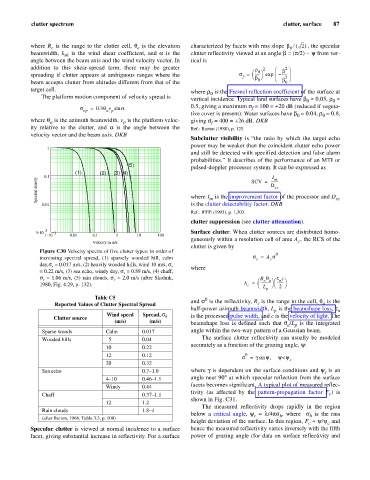
Figure C30 Velocity spectra of five clutter types: in order of 0
increasing spectral spread, (1) sparsely wooded hill, calm s = A s
c
c
day,s v = 0.017 m/s, (2) heavily wooded hills, wind 10 m/s, s v
where
= 0.22 m/s, (3) sea echo, windy day, s v = 0.89 m/s, (4) chaff,
s = 1.06 m/s, (5) rain clouds, s = 2.0 m/s (after Skolnik, æ R q æ t c
v
v
c a ö n ö
--------
1980, Fig. 4.29, p. 132). A = è ------------ ø 2 ø
c
è
L
p
Table C5 0
and s is the reflectivity, R is the range to the cell, q is the
Reported Values of Clutter Spectral Spread c a
half-power azimuth beamwidth, L is the beamshape loss, t n
p
Wind speed Spread, s is the processed pulse width, and c is the velocity of light. The
v
Clutter source
(m/s) (m/s) beamshape loss is defined such that q /L is the integrated
a
p
Sparse woods Calm 0.017 angle within the two-way pattern of a Gaussian beam.
The surface clutter reflectivity can usually be modeled
Wooded hills 5 0.04
accurately as a function of the grazing angle, y:
10 0.22
12 0.12 0
s = g sin y , y<y s
20 0.32

Sea echo 0.7–1.0 where gis dependent on the surface conditions and y is an
s
4–10 0.46–1.1 angle near 90° at which specular reflection from the surface
facets becomes significant. A typical plot of measured reflec-
Windy 0.44
tivity (as affected by the pattern-propagation factor F ) is
Chaff 0.37–1.1 c
shown in Fig. C31.
12 1.2
The measured reflectivity drops rapidly in the region
Rain clouds 1.8–4
below a critical angle, y = l/4ps, where s is the rms
c
h
h
(after Barton, 1964, Table 3.3, p. 100)
height deviation of the surface. In this region, F » y/y and
c
c
Specular clutter is viewed at normal incidence to a surface hence the measured reflectivity varies inversely with the fifth
facet, giving substantial increase in reflectivity. For a surface power of grazing angle (for data on surface reflectivity and