
Page 219 - Radiochemistry and nuclear chemistry
P. 219
Detection and Measurement Techniques 203
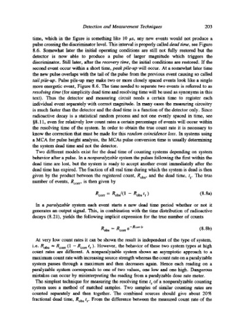
time, which in the figure is something like 10 #s, any new events would not produce a
pulse crossing the discriminator level. This interval is properly called dead time, see Figure
8.6. Somewhat later the initial operating conditions are still not fully restored but the
detector is now able to produce a pulse of larger magnitude which triggers the
discriminator. Still later, after the recovery time, the initial conditions are restored. If the
second event occur within a short time, peak pile-up will occur. At a somewhat later time
the new pulse overlaps with the tail of the pulse from the previous event causing so called
tail pile-up. Pulse pile-up may make two or more closely spaced events look like a single
more energetic event, Figure 8.6. The time needed to separate two events is referred to as
resolving time (for simplicity dead time and resolving time will be used as synonyms in this
text). Thus the detector and measuring circuit needs a certain time to register each
individual event separately with correct magnitude. In many cases the measuring circuitry
is much faster than the detector and the dead time is a function of the detector only. Since
radioactive decay is a statistical random process and not one evenly spaced in time, see
w even for relatively low count rates a certain percentage of events will occur within
the resolving time of the system. In order to obtain the true count rate it is necessary to
know the correction that must be made for this random coincidence loss. In systems using
a MCA for pulse height analysis, the MCAs pulse conversion time is usually dete~ining
the system dead time and not the detector.
Two different models exist for the dead time of counting systems depending on system
behavior after a pulse. In a nonparalyzable system the pulses following the first within the
dead time are lost, but the system is ready to accept another event immediately after the
dead time has expired. The fraction of all real time during which the system is dead is then
given by the product between the registered count, Rob s, and the dead time, t r. The true
number of events, Rcorr, is then given by
Rcorr = Robs/(1 - Rob s tr ) (8.8a)
In a paralyzable system each event starts a new dead time period whether or not it
generates an output signal. This, in combination with the time distribution of radioactive
decays (8.21), yields the following implicit expression for the true number of counts
Robs = Reor r e-Rcorr t, (8.8b)
At very low count rates it can be shown the result is independent of the type of system,
i.e. Rob s ~ Rcorr (1 - Rcorr t r ). However, the behavior of these two system types at high
count rates are different. A nonparalyzable system shows an asymptotic approach to a
maximum count rate with increasing source strength whereas the count rate on a paralyzable
system passes through a maximum and then decreases again. Hence each reading on a
paralyzable system corresponds to one of two values, one low and one high. Dangerous
mistakes can occur by misinterpreting the reading from a paralyzable dose rate meter.
The simplest technique for measuring the resolving time t r of a nonparalyzable counting
system uses a method of matched samples. Two samples of similar counting rates are
counted separately and then together. The combined sources should give about 20%
fractional dead time, Rob s t r. From the difference between the measured count rate of the