Page 147 - Renewable Energy Devices and System with Simulations in MATLAB and ANSYS

134 Renewable Energy Devices and Systems with Simulations in MATLAB and ANSYS ®
®

until sundown. This means that there are periods during the day when the power flows toward the
grid (also called as reverse power flow in the literature) and the house becomes a negative load,
while during peak load periods, the energy is supplied from the grid again. Therefore, it is important
to decide how much power and energy the designed PV system needs to cover, on a daily, monthly,
or even yearly period.

6.2.3 Solar Resource Evaluation

The available sunshine hours will have a direct influence on the payback time of the designed PV
system. In southern Europe, the payback time is around 5–6 years, while in central and northern
Europe, the payback time can reach periods up to 9–10 years or even longer, depending on the local
energy price. This means that the PV system will produce the energy for “free” only after these years
have passed.
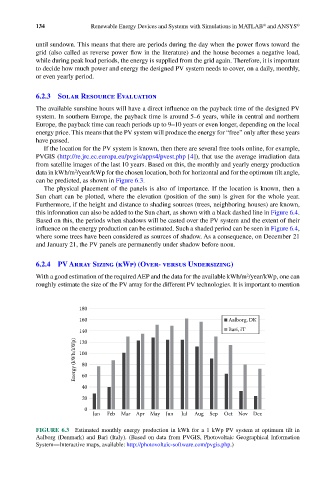
If the location for the PV system is known, then there are several free tools online, for example,
PVGIS (http://re.jrc.ec.europa.eu/pvgis/apps4/pvest.php [4]), that use the average irradiation data
from satellite images of the last 10 years. Based on this, the monthly and yearly energy production
2
data in kWh/m /year/kWp for the chosen location, both for horizontal and for the optimum tilt angle,
can be predicted, as shown in Figure 6.3.
The physical placement of the panels is also of importance. If the location is known, then a
Sun chart can be plotted, where the elevation (position of the sun) is given for the whole year.
Furthermore, if the height and distance to shading sources (trees, neighboring houses) are known,
this information can also be added to the Sun chart, as shown with a black dashed line in Figure 6.4.
Based on this, the periods when shadows will be casted over the PV system and the extent of their
influence on the energy production can be estimated. Such a shaded period can be seen in Figure 6.4,
where some trees have been considered as sources of shadow. As a consequence, on December 21
and January 21, the PV panels are permanently under shadow before noon.

6.2.4 PV Array Sizing (kWp) (Over- versus Undersizing)
With a good estimation of the required AEP and the data for the available kWh/m /year/kWp, one can
2
roughly estimate the size of the PV array for the different PV technologies. It is important to mention

180
160 Aalborg, DK
140 Bari, IT
Energy (kWh/kWp) 100
120

80
60
40
20
0
Jan Feb Mar Apr May Jun Jul Aug Sep Oct Nov Dec

FIGURE 6.3 Estimated monthly energy production in kWh for a 1 kWp PV system at optimum tilt in
Aalborg (Denmark) and Bari (Italy). (Based on data from PVGIS, Photovoltaic Geographical Information
System—Interactive maps, available: http://photovoltaic-software.com/pvgis.php.)