Page 95 - Renewable Energy Devices and System with Simulations in MATLAB and ANSYS

82 Renewable Energy Devices and Systems with Simulations in MATLAB and ANSYS ®
®

4.4.6 Implementation of the Current Controllers
From an implementation point of view, the PI controllers are simple to apply, and any of the dis-
cretization methods (backward Euler, forward Euler, or Tustin) presented earlier can be used. The
implementation of the resonant controllers needs more attention, due to the two parallel-connected
integrators. However, the resonant controller structure is identical with the SOGI implementation
methods given for the SOGI in Section 4.4.4.

4.4.7 Maximum Power Point Tracking
MMPT is one of the essential functions in PV plants. Considering the nonlinear current–voltage
characteristics of PV cells, the maximum power delivered by the PV array is at a well-defined oper-
ating point called maximum power point (MPP). MPPT is one of the key functions that every grid-
connected PV inverter should have. There is a large amount of publications dealing with MPPT, and
trackers in the majority of the commercial PV inverters are able to extract around 99% of the avail-
able power from the PV plant, over a wide irradiance and temperature range—at least in a steady
state. An extensive overview of modern MPPT techniques has been presented in [53]. The most
frequently applied MPPT algorithms are hill-climbing methods, such as the perturb and observe
(P&O), and its alternate implementation (with identical behavior), the incremental conductance
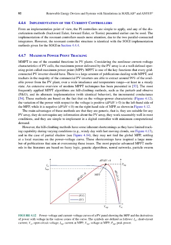
[54]. These methods are based on the fact that on the voltage–power characteristic (Figure 4.12),
the variation of the power with respect to the voltage is positive (dP/dV > 0) in the left-hand side of
the MPP, while it is negative (dP/dV < 0) on the right-hand side of MPP, as shown in Figure 4.12.
The main advantages of these methods are that they are generic, that is, they are suitable for any
PV array, they do not require any information about the PV array, they work reasonably well in most
conditions, and they are simple to implement in a digital controller with minimum computational
demand.
However, the hill-climbing methods have some inherent shortcomings as they have limited track-
ing capability during varying conditions (e.g., windy day with fast moving clouds, see Figure 4.13),
and in the case of partial shadow (see Figure 4.14), they may not find the global MPP, settling
at a local maxima on the power–voltage curve. These shortcomings have inspired a large num-
ber of publications that aim at overcoming these issues. The most popular advanced MPPT meth-
ods in the literature are based on fuzzy logic, genetic algorithms, neural networks, particle swarm

dP/dV=0
I sc P mp
I mp
dP/dV>0 MPP dP/dV< 0

P(V)
I(V)
V mp V oc

FIGURE 4.12 Power–voltage and current–voltage curves of a PV panel showing the MPP and the derivatives
of power with voltage in the various zones of the curve. The symbols are defined as follows: I sc , short-circuit
current; V oc , open-circuit voltage; I mp , current at MPP; V mp , voltage at MPP; P mp , peak power.