Page 91 - Renewable Energy Devices and System with Simulations in MATLAB and ANSYS

78 Renewable Energy Devices and Systems with Simulations in MATLAB and ANSYS ®
®

V΄ α + V΄ α
+
V α 0.5 – V΄ + abc
SOGI-FLL [T ]
–1
qV΄ α V΄ + β αβ
0.5 + +
V abc
[T ]
αβ
V΄ β – V΄ α
–
V β 0.5 + V΄ – abc
–1
SOGI-FLL [T ]
–
qV΄ β 0.5 + + V΄ β αβ
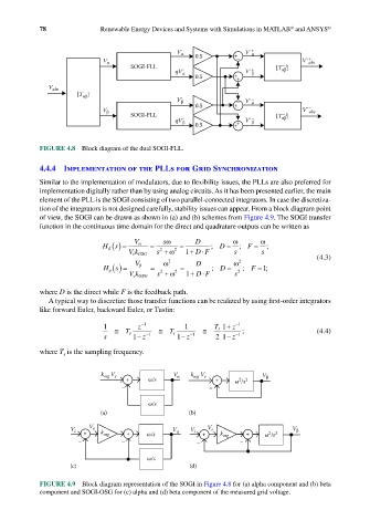
FIGURE 4.8 Block diagram of the dual SOGI-FLL.

4.4.4 Implementation of the PLLs for Grid Synchronization
Similar to the implementation of modulators, due to flexibility issues, the PLLs are also preferred for
implementation digitally rather than by using analog circuits. As it has been presented earlier, the main
element of the PLL is the SOGI consisting of two parallel-connected integrators. In case the discretiza-
tion of the integrators is not designed carefully, stability issues can appear. From a block diagram point
of view, the SOGI can be drawn as shown in (a) and (b) schemes from Figure 4.9. The SOGI transfer
function in the continuous time domain for the direct and quadrature outputs can be written as

Hs () = V α = sω = D ; D = ω ; F = ω ;
d
⋅
2
Vk s + ω 2 1 + DF s s (4.3)
eOSG
ω 2 D ω 2
V β
Hs () = = = ; D = ; F = 1;
q
2 2
⋅
Vk s + ω 2 1+ DF s 2
eOSG
where D is the direct while F is the feedback path.
A typical way to discretize those transfer functions can be realized by using first-order integrators
like forward Euler, backward Euler, or Tustin:
+
1 ≅ z − 1 ≅ 1 ≅ T s 1 z − 1 ; (4.4)
−
−
s T s 1 z− − 1 T s 1 z − 1 2 1 z − 1

where T is the sampling frequency.
s
k V e V k V e V
osg
osg
+ ω/s α + ω /s β
2 2
– –
ω/s
(a) (b)
V i + V e k osg + ω/s V α V i + V e k osg + ω /s V β
2 2
– – – –
ω/s
(c) (d)

FIGURE 4.9 Block diagram representation of the SOGI in Figure 4.8 for (a) alpha component and (b) beta
component and SOGI-OSG for (c) alpha and (d) beta component of the measured grid voltage.