Page 59 - Schaum's Outline of Theory and Problems of Advanced Calculus

50 FUNCTIONS, LIMITS, AND CONTINUITY [CHAP. 3

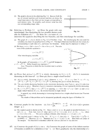
(b) The graph is shown in the adjoining Fig. 3-6. Because both the f (x)
sets of rational numbers and irrational numbers are dense, the
visual impression is that there are two images corresponding to 1
each domain value. In actuality, each domain value has only
one corresponding range value.
x
0
3.4. Referring to Problem 3.1: (a) Draw the graph with axes
Fig. 3-6
interchanged, thus illustrating the two possible choices avail-
1
able for definition of f . (b) Solve for x in terms of y to
determine the equations describing the two branches, and then interchange the variables.
(a) The graph of y ¼ f ðxÞ is shown in Fig. 3-5 of Problem 3.1(a). By interchanging the axes (and the
variables), we obtain the graphical form of Fig. 3-7. This figure illustrates that there are two values of y
corresponding to each value of x, and hence two branches. Either may be employed to define f 1 .
2
(b)We have y ¼ðx 2Þð8 xÞ or x 10x þ 16 þ y ¼ 0. The solu-
tion of this quadratic equation is _
1
y = f (x)
A
8
p ffiffiffiffiffiffiffiffiffiffiffiffi
9 y:
x ¼ 5
6
After interchanging variables P
4
p ffiffiffiffiffiffiffiffiffiffiffi
9 x:
y ¼ 5
2
p ffiffiffiffiffiffiffiffiffiffiffi B
9 x, and BP designates
In the graph, AP represents y ¼ 5 þ
p ffiffiffiffiffiffiffiffiffiffiffi 1 x
9 x. Either branch may represent f .
y ¼ 5
2 4 6 8
Note: The point at which the two branches meet is called a
branch point. Fig. 3-7
ffiffiffiffiffiffiffiffiffiffiffi
p
9 x is strictly decreasing in 0 @ x @ 9. (b)Isit monotonic
3.5. (a)Prove that gðxÞ¼ 5 þ
decreasing in this interval? (c) Does gðxÞ have a single-valued inverse?
(a) gðxÞ is strictly decreasing if gðx 1 Þ > gðx 2 Þ whenever x 1 < x 2 . If x 1 < x 2 then 9 x 1 > 9 x 2 ,
9 x 1 > 9 x 2 ,5 þ 9 x 1 > 5 þ 9 x 2 showing that gðxÞ is strictly decreasing.
ffiffiffiffiffiffiffiffiffiffiffiffiffi ffiffiffiffiffiffiffiffiffiffiffiffiffi ffiffiffiffiffiffiffiffiffiffiffiffiffi ffiffiffiffiffiffiffiffiffiffiffiffiffi
p p p p
(b)Yes, any strictly decreasing function is also monotonic decreasing, since if gðx 1 Þ > gðx 2 Þ it is also true
that gðx 1 Þ A gðx 2 Þ. However, if gðxÞ is monotonic decreasing, it is not necessarily strictly decreasing.
p ffiffiffiffiffiffiffiffiffiffiffi p ffiffiffiffiffiffiffiffiffiffiffi 2
(c) If y ¼ 5 þ 9 x,then y 5 ¼ 9 x or squaring, x ¼ 16 þ 10y y ¼ðy 2Þð8 yÞ and x is a
single-valued function of y, i.e., the inverse function is single-valued.
In general, any strictly decreasing (or increasing) function has a single-valued inverse (see Theorem
6, Page 47).
The results of this problem can be interpreted graphically using the figure of Problem 3.4.

x sin 1=x; x > 0
3.6. Construct graphs for the functions (a) f ðxÞ¼ 0; x ¼ 0 , (b) f ðxÞ¼½xŠ¼ greatest
integer @ x.
(a) The required graph is shown in Fig. 3-8. Since jx sin 1=xj @ jxj,the graph is included between y ¼ x
and y ¼ x. Note that f ðxÞ¼ 0 when sin 1=x ¼ 0or1=x ¼; m , m ¼ 1; 2; 3; 4; ... ; i.e., where
x ¼ 1= ; 1=2 ; 1=3 ; ... . The curve oscillates infinitely often between x ¼ 1= and x ¼ 0.
p ffiffiffi
(b) The required graph is shown in Fig. 3-9. If 1 @ x < 2, then ½xŠ¼ 1. Thus ½1:8Š¼ 1, ½ 2Š¼ 1,
½1:99999Š¼ 1. However, ½2Š¼ 2. Similarly for 2 @ x < 3, ½xŠ¼ 2, etc. Thus there are jumps at
the integers. The function is sometimes called the staircase function or step function.
3.7. (a) Construct the graph of f ðxÞ¼ tan x.(b) Construct the graph of some of the infinite number
1
of branches available for a definition of tan x.(c) Show graphically why the relationship of x