Page 62 - Schaum's Outline of Theory and Problems of Electric Circuits

CHAP. 4]
Similarly, ANALYSIS METHODS 51

N 2 1700 N 3 5600
I 2 ¼ ¼ ¼ 3:17 A I 3 ¼ ¼ ¼ 10:45 A
R 536 R 536

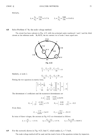
4.8 Solve Problem 4.7 by the node voltage method.
The circuit has been redrawn in Fig. 4-22, with two principal nodes numbered 1 and 2 and the third
chosen as the reference node. By KCL, the net current out of node 1 must equal zero.

Fig. 4-22

V 1 25
V 1 V 1 V 2
þ þ ¼ 0
2 5 10
Similarly, at node 2,
V 2 þ 50
V 2 V 1 V 2
þ þ ¼ 0
10 4 2
Putting the two equations in matrix form,
2 32 3
1 1 1 1 5
6 2 þ þ 10 10 76 V 1 7
5
6 76 7 ¼
4 1 1 1 1 54 5
þ þ V 2 25
10 10 4 2
The determinant of coefficients and the numerator determinants are

0:80 0:10
¼ 0:10 0:85 ¼ 0:670

5 0:10 0:80 5
N 1 ¼ 25 0:85 ¼ 1:75 N 2 ¼ 0:10 25 ¼ 19:5
From these,
1:75 19:5
V 1 ¼ ¼ 2:61 V V 2 ¼ ¼ 29:1V
0:670 0:670
In terms of these voltages, the currents in Fig. 4-21 are determined as follows:
V 1 V 1 V 2 V 2 þ 50
I 1 ¼ ¼ 1:31 A I 2 ¼ ¼ 3:17 A I 3 ¼ ¼ 10:45 A
2 10 2

4.9 For the network shown in Fig. 4-23, find V s which makes I 0 ¼ 7:5 mA.
The node voltage method will be used and the matrix form of the equations written by inspection.