Page 127 - Science at the nanoscale

RPS: PSP0007 - Science-at-Nanoscale
8:11
June 9, 2009
6.1. From 3D to 0D Nanostructures
1.2
g
(E)
c
1.0
E F
States
ƒ(E)
0.8
Probability
n(E)
of
0.6
Density
0.4
0.2
0
Energy (eV)
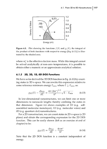
Plot showing the functions f (E) and g c (E); the integral of
Figure 6.5.
the product of both functions with respect to energy [Eq. (6.11)] is illus-
trated by the shaded area.
where m is the effective electron mass. While this integral cannot
∗
e
be solved analytically at non-zero temperatures, it is possible to
obtain either a numeric or an approximate analytical solution.
6.1.3
3D, 2D, 1D, 0D DOS Functions
We have so far derived the 3D DOS function in Eq. (6.10) by count-
ing states in 3D n-space. We can rewrite this expression relative to
some reference minimum energy E min , where E ≥ E min , as:
∗ 3/2
4π (2m )
dn 3D
p
(6.13)
=
E − E min
g 3D (E) =
3
dE
h
In low-dimensional nanostructures, we can limit one or more
dimensions to nanoscale lengths thereby confining the states in
that dimension. Figure 6.6 shows examples of 2D (e.g. self- 117 ch06
assembled molecular monolayer), 1D (e.g. molecular wires) and
0D (e.g. quantum dot) nanostructures.
For a 2D nanostructure, we can count states in 2D n-space (a 2D
plane) and obtain the corresponding expression for the 2D DOS
function. This can be easily shown (left as an exercise at end of
chapter) to be:
4πm ∗
dn 2D
g 2D (E) = = 2 (6.14)
dE h
Note that the 2D DOS function is a constant independent of
energy.