Page 129 - Science at the nanoscale

RPS: PSP0007 - Science-at-Nanoscale
8:11
June 9, 2009
6.1. From 3D to 0D Nanostructures
1D
2D
3D
0D
(Quantum Well)
(Quantum Wire)
(bulk)
(Quantum Dot)
g(E)
g(E)
g(E)
g(E)
E
E
E
E
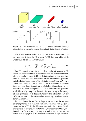
Density of states for 3D, 2D, 1D, and 0D structures showing
Figure 6.7.
discretization of energy levels and discontinuity in the density of states.
For a 1D nanostructure such as the carbon nanotube, we
can also count states in 1D n-space (a 1D line) and obtain this
expression for the 1D DOS function:
r
1
2m
∗
dn 1D
(6.15)
√
=
g 1D (E) =
2
h
dE
E − E min
In a 0D nanostructure, there is only one discrete energy in 0D
space. All the available states therefore exist only at discrete ener-
gies and can be represented by a delta function. In real quantum
dots, however, the size distribution of the ensemble of quantum
dots leads to a broadening of this delta function. Figure 6.7 shows
schematics of the 3D, 2D, 1D and 0D DOS functions. Note that
there may be different quantised levels in low dimensional nanos- 119 ch06
tructures, e.g. even though the 2D DOS is constant for a quantum
well, it is usually a step function with steps occurring at the energy
of each quantized level. Figure 6.8 shows the calculated DOS for
different types of carbon nanotubes, revealing the characteristic
1D DOS features.
Table 6.2 shows the number of degenerate states for the ten low-
est energy levels in a quantum well (2D), quantum wire (1D) and
quantum box (0D). In the 2D quantum well, the ratio of the ith
2
energy level to the ground state level E 0 is proportional to n , and
in each case there is only one way in which n can be arranged to
obtain this energy; hence the degeneracy of each energy level is 1.