Page 145 - Separation process principles 2

110 Chapter 3 Mass Transfer and Diffusion

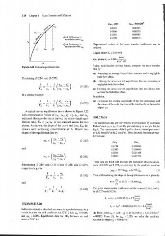
xiis a fictitious xA in
equilibrium with ynb

yiis a fictitious yA in Experimental values of the mass transfer coefficients are as
equilibrium with xAb
follows.
Liquid phase: kc = 0.18 m/h
kmol
Gas phase: kp = 0.040------
h-m2-k~a
IA
Using mole-fraction driving forces, compute the mass-transfer
Figure 3.22 Curved equilibrium line.
flux by:
(a) Assuming an average Henry's-law constant and a negligible
bulk-flow effect.
Combining (3-234) and (3-237),
(b) Utilizing the actual curved equilibrium line and assuming a
negligible bulk-flow effect.
(c) Utilizing the actual curved equilibrium line and taking into
account the bulk-flow effect.
In a similar manner,
In addition,
(d) Determine the relative magnitude of the two resistances and
the values of the mole fractions at the interface from the results
of part (c).
A typical curved equilibrium line is shown in Figure 3.22
with representative values of YA~, YA, , y;, xi;, XA,, and XA,
indicated. Because the line is curved, the vapor-liquid equi- SOLUTION
librium ratio, KA = yA/xA, is not constant across the two The equilibrium data are converted to mole fractions by assuming
phases. As shown, the slope of the curve and thus, KA, de- Dalton's law, y~ = pA/P, for the gas and using XA = cA/c for the
creases with increasing concentration of A. Denote two liquid. The concentration of the liquid is close to that of pure water
slopes of the equilibrium line by or 3.43 lbmol/ft3 or 55.0 kmoUm3. Thus, the mole fractions at equi-
librium are:

and

These data are fitted with average and maxinlum absolute devia-
Substituting (3-240) and (3-241) into (3-238) and (3-239), tions of 0.91% and 1.16%, respectively, by the quadratic equation
respectively, gives

Thus, differentiating, the slope of the equilibrium curve is given by

and
The given mass-transfer coefficients can be converted to k, and k,
by (3-227) and (3-228):
kmol
k, = kCc = 0.18(55.0) = 9.9-
h-m2
EXAMPLE 3.20 kmol
k, = kp P = 0.040(2)(101.3) = 8.1 -
Sulfur dioxide (A) is absorbed into water in a packed column. At a h-m2 '
certain location, the bulk conditions are 50°C, 2 atm, y~~ = 0.085, (a) From (1) forx~, = 0.001, yi = 29.74(0.001) + 6,733(0.001)~
and XA~ = 0.001. Equilibrium data for SO2 between air and = 0.0365. From (I), for y~, 0.085, we solve the quadratic
=
water at 50°C are equation to obtain xi = 0.001975.