Page 140 - Separation process principles 2

3.6 Models for Mass Transfer at a Fluid-Fluid Interface 105

[ following form of (3-79): Surface-Renewal Theory

The penetration theory is not satisfying because the as-
sumption of a constant contact time for all eddies that tem-
porarily reside at the surface is not reasonable, especially
for stirred tanks, contactors with random packings, and
bubble and spray columns where the bubbles and droplets
[ ~hus, the penetration theory gives cover a wide range of sizes. In 1951, Danckwerts [60] sug-
gested an improvement to the penetration theory that
involves the replacement of the constant eddy contact
time with the assumption of a residence-time distribution,
wherein the probability of an eddy at the surface being
which predicts that kc is proportional to the square root of the
replaced by a fresh eddy is independent of the age of the
molecular diffusivity, which is at the lower limit of experi- surface eddy.
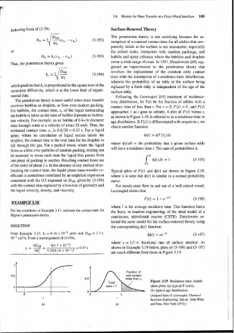
mental data. Following the Levenspiel [6 I] treatment of residence-
The penetration theory is most useful when mass transfer
time distribution, let F(t) be the fraction of eddies with a
involves bubbles or droplets, or flow over random packing.
contact time of less than t. For t = 0, F{t} = 0, and F{t)
For bubbles, the contact time, tc, of the liquid surrounding
approaches 1 as t goes to infinity. A plot of F(t) versus t,
the bubble is taken as the ratio of bubble diameter to bubble- as shown in Figure 3.19, is referred to as a residence-time or
rise velocity. For example, an air bubble of 0.4-cm diameter
age distribution. If Fit) is differentiated with respect to t, we
rises through water at a velocity of about 20 crnls. Thus, the obtain another function:
estimated contact time, tc, is 0.4/20 = 0.02 s. For a liquid
spray, where no circulation of liquid occurs inside the
droplets, the contact time is the total time for the droplets to
where +{t}dt = the probability that a given surface eddy
fall through the gas. For a packed tower, where the liquid
will have a residence time t. The sum of probabilities is
flows as a film over particles of random packing, mixing can
be assumed to occur each time the liquid film passes from
one piece of packing to another. Resulting contact times are
of the order of about 1 s. In the absence of any method of es-
timating the contact time, the liquid-phase mass-transfer co- Typical plots of F(t) and +(t] are shown in Figure 3.19,
efficient is sometimes correlated by an empirical expression where it is seen that +It} is similar to a normal probability
consistent with the 0.5 exponent on DAB, given by (3-194) curve.
with the contact time replaced by a function of geometry and For steady-state flow in and out of a well-mixed vessel,
the liquid velocity, density, and viscosity. Levenspiel shows that

F{t) = 1 - e-'li (3-196)
where f is the average residence time. This function forms
For the conditions of Example 3.17, estimate the contact time for
the basis, in reaction of the ideal model of a
Higbie's penetration theory.
continuous, stirred-tank reactor (CSTR). Danckwerts se-
lected the same model for his surface-renewal theory, using
SOLUTION the corresponding +(t} function:

From Example 3.17, kc = 6.14 x cm/s and DAB = 1.7 x ${t) = sePSt (3-197)
lop5 cm2/s. From a rearrangement of (3-194),
where s = l/i = fractional rate of surface renewal. As
4DAB 4(1.7 X
1 C - - = 0.57 s shown in Example 3.19 below, plots of (3-196) and (3-197)
~k: 3.14(6.14 x 10-3)2
are much different from those in Figure 3.19.

IA

F{t)
older than t,
Total . . Figure 3.19 Residence-time distrib-
0 1 ------+--------- area = 1 ution plots: (a) typical F curve;
I > (b) typical age distribution.
I
0 t 0 f 1 [Adapted from 0. Levenspiel, Chemical
t t
Reaction Engineering, 2nd ed., John Wiley
(a) (b) and Sons, New York (1972).]