Page 154 - Separation process principles 2

4.2 Binary Vapor-Liquid Systems 119

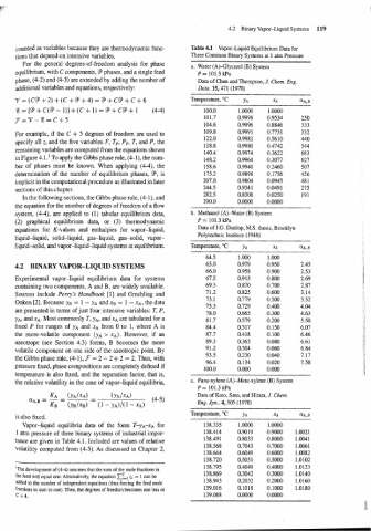
counted as variables because they are thermodynamic func- Table 4.1 Vapor-Liquid Equilibrium Data for
tions that depend on intensive variables. Three Common Binary Systems at 1 atm Pressure
For the general degrees-of-freedom analysis for phase a. Water (A)-Glycerol (B) System
equilibrium, with C components, 9 phases, and a single feed P = 101.3 kPa
phase, (4-2) and (4-3) are extended by adding the number of Data of Chen and Thompson, J. Chem. Eng.
additional variables and equations, respectively: Data, 15,471 (1970)

Temperature, OC

For example, if the C + 5 degrees of freedom are used to
specify all zi and the five variables F, TF, PF, T, and P, the
remaining variables are computed from the equations shown
in Figure 4.1.' To apply the Gibbs phase rule, (4-l), the num-
ber of phases must be known. When applying (4-4), the
determination of the number of equilibrium phases, 9, is
implicit in the computational procedure as illustrated in later
sections of this chapter.
In the following sections, the Gibbs phase rule, (4-l), and
the equation for the number of degrees of freedom of a flow
system, (4-4), are applied to (1) tabular equilibrium data, b. Methanol (A)-Water (B) System
(2) graphical equilibrium data, or (3) thermodynamic P = 101.3 kPa
equations for K-values and enthalpies for vapor-liquid, Data of J.G. Dunlop, M.S. thesis, Brooklyn
Polytechnic Institute (1948)
liquid-liquid, solid-liquid, gas-liquid, gas-solid, vapor-
liquid-solid, and vapor-liquid-liquid systems at equilibrium. Temperature, "C yA XA ~A,B

4.2 BINARY VAPOR-LIQUID SYSTEMS
Experimental vapor-liquid equilibrium data for systems
containing two components, A and B, are widely available.
Sources include Perry's Handbook [I] and Gmehling and
Onken [2]. Because y~ = 1 - y~ and XB = 1 - XA, the data
are presented in terms of just four intensive variables: T, P,
y~, and XA. Most commonly T, y~, and XA are tabulated for a
fixed P for ranges of y~ and XA from 0 to 1, where A is
the more-volatile component (yA > xA). However, if an
azeotrope (see Section 4.3) forms, B becomes the more
volatile component on one side of the azeotropic point. By
the Gibbs phase rule, (4-I), 3 = 2 - 2 + 2 = 2. Thus, with
pressure fixed, phase compositions are completely defined if
temperature is also fixed, and the separation factor, that is,
the relative volatility in the case of vapor-liquid equilibria, c. Para-xylene (A)-Meta-xylene (B) System
P = 101.3 kPa
Data of Kato, Sato, and Hirata, J. Chem.
Eng. Jpn., 4,305 (1970)
-
Temperature, "C y~ XA ~A,B
is also fixed.
Vapor-liquid equilibria data of the form T-y~-XA for 138.335 1 .OOOO 1 .OOOO
1 atm pressure of three binary systems of industrial impor- 138.414 0.9019 0.9000 1.0021
tance are given in Table 4.1. Included are values of relative 138.491 0.8033 0.8000 1.0041
volatility computed from (4-5). As discussed in Chapter 2, 138.568 0.7043 0.7000 1.0061
138.644 0.6049 0.6000 1.0082
138.720 0.5051 0.5000 1.0102
138.795 0.4049 0.4000 1.0123
'The development of (4-4) assumes that the sum of the mole fractions in
138.869 0.3042 0.3000 1.0140
the feed will equal one. Alternatively, the equation zE1 zi = 1 can be
138.943 0.2032 0.2000 1.0160
added to the number of independent equations (thus forcing the feed mole
fractions to sum to one). Then, the degrees of freedom becomes one less or 139.016 0.1018 0.1000 1.0180
c+4. 139.088 0.0000 0.0000
(I!
1I1lI