Page 156 - Separation process principles 2

4.2 Binary Vapor-Liquid Systems 121

Mole fraction of methanol in liquid, x, or vapor, y Mole fraction of methanol in liquid
(a) (b)

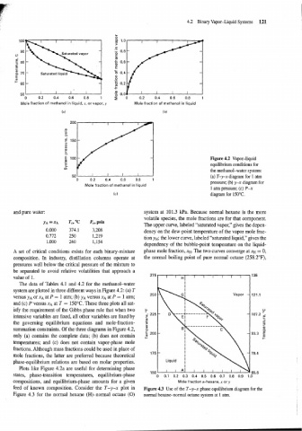
Figure 4.2 Vapor-liquid
equilibrium conditions for
the methanol-water system:
501 I I I I (a) T-y-x diagram for 1 atm
0 0.2 0.4 0.6 0.8 1
pressure; (b) y-x diagram for
Mole fraction of methanol in liquid
1 atrn pressure; (c) P-x
(c) diagram for 150°C.

and pure water: system at 101.3 kPa. Because normal hexane is the more
volatile species, the mole fractions are for that component.
y~ =XA Tc, OC PC, psia
The upper curve, labeled "saturated vapor," gives the depen-
0.000 374.1 3,208 dency on the dew-point temperature of the vapor mole frac-
0.772 250 1,219
tion y~; lower curve, labeled "saturated liquid," gives the
the
1 .OOO 240 1,154
dependency of the bubble-point temperature on the liquid-
A set of critical conditions exists for each binary-mixture phase mole fraction, XH. The two curves converge at XH = 0,
composition. In industry, distillation columns operate at the normal boiling point of pure normal octane (258.2"F),
pressures well below the critical pressure of the mixture to
be separated to avoid relative volatilities that approach a
275 I I 135
value of 1.
" 1 " 1 1 1 1
The data of Tables 4.1 and 4.2 for the methanol-water I
system are plotted in three different ways in Figure 4.2: (a) T
Vapor - 121.1
versus y~ or XA at P = 1 atm; (b) y~ versus XA at P = 1 atm;
and (c) P versus XA at T = 150°C. These three plots all sat-
isfy the requirement of the Gibbs phase rule that when two +
intensive variables are fixed, all other variables are fixed by
the governing equilibrium equations and mole-fraction-
summation constraints. Of the three diagrams in Figure 4.2,
only (a) contains the complete data; (b) does not contain
temperatures; and (c) does not contain vapor-phase mole
fractions. Although mass fractions could be used in place of 175 -
mole fractions, the latter are preferred because theoretical
phase-equilibrium relations are based on molar properties.
Plots like Figure 4.2a are useful for determining phase
states, phase-transition temperatures, equilibrium-phase o 0.1 0.2 0.3 0.4 0.5 0.6 0.7 0.8 0.9 1.0
~orn~oshions, and equilibrium-phase amounts for a given Mole fraction n-hexane, x or y
feed of known composition. Consider the T-Y-x plot in Figure 4.3 Use of the T-y-x phase equilibrium diagram for the
Figure 4.3 for the normal hexane (H)-normal octane (0) normal hexane-normal octane system at 1 atm.