Page 145 - Six Sigma Demystified

126 Six SigMa DemystifieD

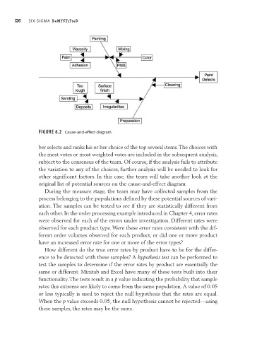
Figure­6.2 Cause- and- effect diagram.

ber selects and ranks his or her choice of the top several items. The choices with
the most votes or most weighted votes are included in the subsequent analysis,
subject to the consensus of the team. Of course, if the analysis fails to attribute
the variation to any of the choices, further analysis will be needed to look for
other significant factors. In this case, the team will take another look at the
original list of potential sources on the cause- and- effect diagram.
During the measure stage, the team may have collected samples from the
process belonging to the populations defined by these potential sources of vari-
ation. The samples can be tested to see if they are statistically different from
each other. In the order processing example introduced in Chapter 4, error rates
were observed for each of the errors under investigation. Different rates were

observed for each product type. Were these error rates consistent with the dif-
ferent order volumes observed for each product, or did one or more product
have an increased error rate for one or more of the error types?
How different do the true error rates by product have to be for the differ-
ence to be detected with these samples? A hypothesis test can be performed to
test the samples to determine if the error rates by product are essentially the
same or different. Minitab and Excel have many of these tests built into their
functionality. The tests result in a p value indicating the probability that sample
rates this extreme are likely to come from the same population. A value of 0.05
or less typically is used to reject the null hypothesis that the rates are equal.
When the p value exceeds 0.05, the null hypothesis cannot be rejected— using
these samples, the rates may be the same.