Page 216 - Six Sigma Demystified

196 Six SigMa DemystifieD

Standard control charts require that observations from the process are indepen-
dent of one another. Failure to meet this requirement increases the chance that
the control chart will falsely indicate a process shift. Therefore, the autocorrela-
tion function is a good tool to use to check the independence assumption. If
control limits on an X chart are particularly tight, with many out-of-control
points, autocorrelation should be suspected.
Many of the statistical tools, including regression, ANOVA, and general
hypothesis tests, assume independence of the data observations. Failure to sat-
isfy this assumption may result in increased type I and type II errors. Autocor-
relation is inherent to many processes, including

• Chemical processes. Here, autocorrelation occurs because of the inertia of
large batches, the continuous flow of material, and/or feedback and feed-
forward process control systems.

• Service processes. As described in queuing theory, wait times for customers
are often influenced by the wait time of previous customers.

• Manufacturing processes. Here, autocorrelation occurs because of com-
puter control of production equipment and downstream pooling of mul-
tiple-stream processes.

Methodology

The ACF will first test whether adjacent observations are autocorrelated,
that is, whether there is correlation between observations 1 and 2, 2 and 3,
3 and 4, and so on. This is known as lag 1 autocorrelation because one of the
pairs of tested observations lags the other by one period or sample. Similarly,

it will test at other lags. For instance, the autocorrelation at lag 4 tests,
whether observations 1 and 5, 2 and 6, . . . , 19 and 23, and so on, are cor-
related.
In general, we should test for autocorrelation at lag 1 to lag n/4, where n is
the total number of observations in the analysis. Estimates of longer lags have
been shown to be statistically unreliable (Box and Jenkins, 1970).

Autocorrelation Function
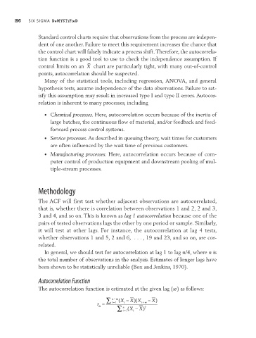
The autocorrelation function is estimated at the given lag (w) as follows:

∑ n − m m m ( ( X − X X− X ) ) )( ( ( X − X) ) )
−
−
i =1 X X(
n
X X
n −
− X− X
i
i i i
i + m m
i +
i =1
r = = = ∑ ∑ i =1 ∑ i =1 X( ( (X i i i X) ) ) + m 2 2 2
m r r
m m
X − X− X−
n n n
∑ ∑ i =1
i =1